BrainVoyager v23.0
Single-Subject GLM Analysis
This section describes how data from a single subject can be analyzed with the General Linear Model (GLM). To understand the concepts behind the GLM, consult sections Principles of Statistical Data Analysis and The General Linear Model. A more detailled step-by-step description on how to use BrainVoyager to perform single-subject GLM analyses can be found in the BrainVoyhager Getting Sarted Guide (steps 6 and 14).
Prerequisites
In order to analyze a run of a subject, a functional time course data file must be available. Depending on the space of the data, this can be an FMR (set of slices in original (scanned) orientation), VMR-VTC (full 3D space, typically in MNI or Talairach space) or SRF-MTC (typically cortex space) data set. Besides the voxel time course data, a protocol file should be available for the respective run. A protocol file forms the basis for the automatic definition of a design matrix X for the time course data of a single run (one functional scan of potentially several ones in a session). A protocol file can be easily created and linked to the respective functional time course data. If the time course data is saved after establishing the link to the protocol, it will be automatically available in future cases when the functional data is reloaded. While very helpful, a protocol file is not absolutely necessary since the design matrix for the run can also be built for defined intervals interactively. In the following it is assumed that a volume time course (VTC) data set is available that contains a link to a protocol. The sample data used is from the Getting Started Guide "Objects" data.
Linking Time Course Data
For FMR-STC data, the time course data and the (pseudo-)anatomical data are available and a GLM can be calculated immediately. For VMR-VTC and SRF-MTC data, a time course must be linked to the VMR document or mesh document, respectively. For a single-run VMR-VTC GLM shown below, a volume time course (VTC) file needs to be linked to a VMR file in a matching reference space.
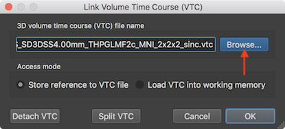
In the snapshot above, the Browse button in the Link Volume Time Course (VTC) dialog has been used to associate a .vtc file in MNI space to the VMR data of the respective subject in MNI space (see below). A qucker way to link a VTC file is to click the Link VTC item in the document context menu that is available by right-clicking on the title bar of the VMR document window, which will directly show a File Open dialog to select the VTC file. Having a VTC file associated with the current VMR document, a single-run GLM can now be performed using the Single Study General Linear Model dialog that can be invoked by clicking the Single Study General Linear Model item in the Analysis menu, or by clicking the Singe-Run GLM item from the document's context menu.
Automatic Definition of Design Matrix
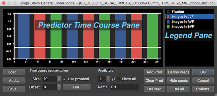
Since a block design protocol had been previously linked to the VTC data, the protocol generated for this subject will be shown in the dialog's Predictor Time Course pane automatically (see above). The display shows that each block of three main conditions ("Images in LVF", "Images in RVF", "Images in BVF") occurrs three times in the protocol. Furthermore, a baseline conditon is inserted between all main conditions. The name and colors of each protocol condition is shown in the Legend Pane on the right. A horizontal white line appears in the predictor time course window indicating one predictor time course of the (not yet defined) design matrix with only "0" values at each time point ("empty" predictor). The most convenient way to generate a design matrix requires only clicking the Define Preds button (see arrow in the screenshot below).
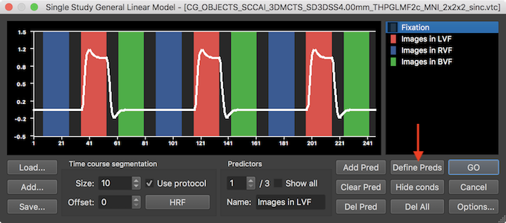
This will automatically define one predictor time course for each of the three main conditions but not for the first ("Fixation") condition, which is usually considered as a baseline (for more details, see below). To calculate the GLM with the automatically defined design matrix, the GO button can be clicked to obtain statistical maps overlaid on the anatomical VMR document.
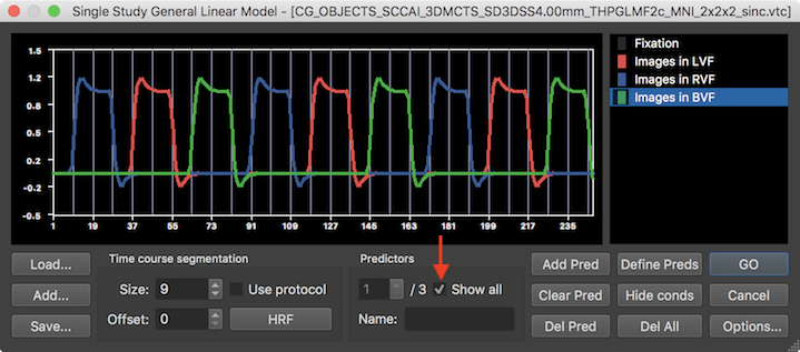
When defining the design matrix automatically using the Define Preds button, two internal steps are performed to generate each predictor time course. In the first internal step, the time intervals belonging to a condition are defined as a "box car" time course (value "1" for time points falling in a condition interval, value "0" for time points not included in the condition). In the second internal step, the generated box-car time course is convolved with the default (two-gamma) hemodynamic response function to get the displayed gradually changing predictor time courses. The predictor time courses can be inspected by changing the value in the Predictors spin box. The name of a predictor is shown in the Name text box of the Predictors field; as default, the name of a predictor corresponds to the corresponding name of the protocol condition but it may be edited if desired. Clicking the Show all option will superimpose all individual predictor time courses (see snapshto below).
Note that the set of intervals defining the first condition ("Fixation" in the example data) is not modelled with a predictor in order to keep the design matrix non-singular. Dropping the first condition (interpreted as "baseline") from the design matrix implements a default assumption, which can be changed in the Single Study GLM Options dialog, which can be invoked by clicking the Options button in the right lower corner. For later use, one can save the defined design matrix by using the Save button on the left side (e.g. as "sub-01_task-VisualExperiment.sdm"). The availablility of a design matrix (SDM, single-run design matrix) file is especially important for building multi-run / multi-subject (MDM) design matrices later. For this reason, the design matrix is also auto-saved to disk with a file name corresponding to the functional time course (e.g. VTC) by replacing its file extension with the "_autosave.sdm" substring.

To calculate a GLM (including estimation of beta values) for each voxel of the single-run data, click the GO button. When calculations are finished, the program automatically overlays the resulting statistical parametric map using a default contrast with all conditions "turned on".
Manual Definition of Design Matrix
[coming soon]
alternatively you may also load a previously saved design matrix file using the Load button on the left side.
Copyright © 2023 Rainer Goebel. All rights reserved.