BrainVoyager v23.0
pRF Estimation in Volume Space
The Fit pRFs tab of the Population Receptive Field dialog is used to find the population receptive field model that best explains the measured fMRI time courses of provided input data. If the dialog is called from a VMR document window, the Fit pRFs tab adjusts some of its fields to VMR-VTC projects. To run the pRF fitting procedure, the program needs as one input source the model time course created earlier with the Stimulus Time Courses tab. The Load button on the right side of the Predicted time courses text field (see snapshot below) can be used to load a desired .ptc file; note that this field might be already filled in case one moves straight to the Fit pRFs tab after having generated time courses in the Stimulus Time Courses tab.
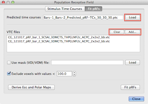
Furthermore, the program needs to know the VTC files that contain the measured fMRI time course data. One or more VTC files can be added to the VTC files list using the Add button (see snapshot above). Note that the pRF scanning included multiple runs, the order in which the VTC files are added here needs to match the order in which the stimuli have been added in the Stimulus Time Courses tab to generate the .stm file. For the used example, two VTC files have been added containing the measured fMRI data of the two experimental runs where bar stimuli had been presented.
Since all (e.g. 27,000) model time courses are fitted in separate GLM's to each voxel of the VMR-VTC project, it is recommended to limit the number of considered voxels to those in a mask containing the grey matter of the occipital lobe. Voxels can be restricted to voxels that are specified in a region-of-interest. The Load button on the right side of the Use mask (VOI/VOM) file text field (see snapshot below) can be used to load a previously prepared region-of-interest file that can be either a .voi or .vom file. One possibility to get a useful grey matter mask is to run a standard GLM contrasting stimulation periods to baseline (fixation) periods. This requires creation of a corresponding protocol (.prt) file; the resulting statistical map can be converted into a single VOI by using the Convert Map to VOIs dialog (accessible via the Options menu). It is also possible to use segmentation tools to get a VOI containing grey matter voxels and to restrict them roughly to the occipital lobe; if a cortex mesh is available, the Create Cortex-Based VTC Mask dialog (accessible in the Meshes menu) can be used to get a grey matter mask that can be further refined to only contain grey matter voxels in the posterior part of the brain and then converted to a VOI. It is generally worth to create such a mask since it will substantially reduce calculation time.
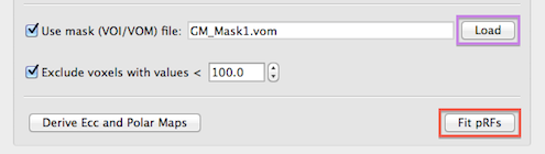
If a VOI file is used as a mask, the voxel coordinates (specified in the resolution of the anatomical VMR data) will be converted internally to the resolution of the used functional (VTC) data. If a VOM file is used, the voxels are already specified in the same resolution as the functional data and used as defined in the .vom file. If you have defined a VOI file, you can use it directly or use the Create VOMs dialog to convert the defined VOI into a VOM region-of-interest. Note that it is recommended to have only one ROI defined in the .voi file - if more than one ROI is available, only the first one will be used. Besides spatial masking, voxels can also be excluded if they contain time course data with low intensity values likely corresponding to non-brain background voxels. This exclusion criteria is enabled by checking the Exclude voxels with values < option (turned on as default) and the threshold intensity value can be specified in the Intensity threshold spin box (value 100.0 is used as a reaonable default setting). While this option (see snapshot above) is not relevant when using a cortex mask, it helps to reduce the number of analyzed voxels when no VOI/VOM file is provided.
If the pRF model time course data, the VTC file(s) and optionally a spatial mask file have been provided as input, the population receptive field estimation can be started by clicking the Fit pRFs button (see snapshot above). For each voxel included in the analysis, a separate GLM is executed for each pRF model with the model's time course as the main predictor (predictor of interest) of the GLM design matrix X. For each run included in the analysis, a separate constant predictor is added to the design matrix (as in a multi-run GLM) allowing to fit a different beta weight for the baseline level. The voxel's time course data is transformed into percent signal change values separately for each run and then concatenated providing the observed (to-be-explained) data y of the GLM. The GLM for each pRF model is calculated and the amount of explained variance R2 is recorded - the model that results in a GLM with the highest explained variance value is assigned as the pRF model for the considered voxel. This procedure is repeated for each voxel included in the analysis. The parameters of the best fitting model are stored in a volume map providing the final output of the fitting procedure, i.e. for each analyzed voxel, the pRF model's position in the visual field (x, y values) and the model's receptive field size are recorded in different sub-maps (see snapshots below) of the volume map data. The volume map is saved to disk automatically using an appropriate name containing the name of the mask file (if used) and number and range of pRF models used (i.e. the name will be similar as the one created for the .ptc file).
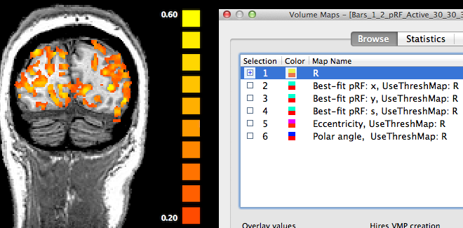
In order to inspect the estimated pRF data, open the Volume Maps dialog (see snapshot above). The dialog will contain six sub-maps. The first sub-map is a multiple correlation map named "R" (see snapshot above) containing the square root of the explained variance of the best fitting pRF model per voxel. This statistical map is instructive in itself but it is also used to theshold other maps that contain non-statistical values such as the location of the voxel's pRF in the visual field. Note that all other sub-maps contain the sub-string "UseThreshMap: R" in the map name. The "UseThreshMap" instruction string has been originally introduced in the context of "winner maps" to allow sub-maps containing qualitative (non-ordered categorical) values to use another map for thresholding. This mechanism has been extended to support that any kind of map can refer to any other map using it for thresholding. This provides the possibility for pRF model parameter maps as well as derived eccentricity and polar angle maps (see below) to show the full range of their values while still being able to remove noisy voxels by using the "R" map for thresholding. If the threshold (set to 0.2 as default) of the "R" map is changed, the effect will be visible when selecting one of the other sub-maps.
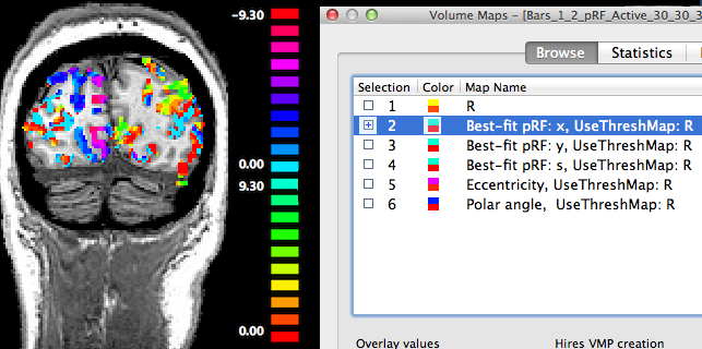
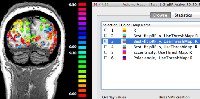
The second map "Best-fit pRF: x" contains the x location of the pRF model assigned to a voxel. As one would expect, positive x values (representing pRF model locations in the right visual field) are visible in the brain mainly in the left hemisphere (shown on the right side in the displayed radiologcial convention) and negative x values (left visual field) are shown mainly in the right hemisphere (see snapshot above).
The third map "Best-fit pRF: y" contains the y location of the pRF model assigned to a voxel. In the snapshot above mainly positive values (red-yellow-green colors) are visible since the selected coronal cut contains mainly visual cortex for lower visual field locations.
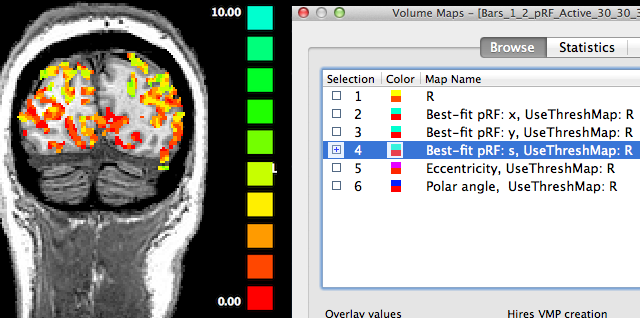
The fourth map "Best-fit pRF: s" contains the receptive field size of the pRF model assigned to a voxel. The red/orange colors in the lower medial part of the cortex shown in the snapshot above indicate that receptive field sizes are small in these regions while in the more lateral upper parts of the visible cortex contain larger receptive field sizes as indicated by the yellow/green colors. Note that it may be instructive to change the upper (display) threshold to a lower value than the default value in order to better see small gradients of receptive field size changes, e.g. within areas V1/V2.
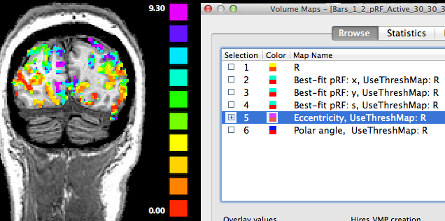
The maps described so far are direct representations of the population receptive field models fitted to the data. Sub-maps 5 and 6 contain eccentricity and polar angle values that are simply derived from the x and y pRF model parameter maps. These maps are added to provide visualizations of the obtained pRF results in the same way as in conventional phase-encoded retinotopic mapping experiments. The fifth map "Eccentricity" contains estimates of eccentricity values ecc that are simply obtained by applying the equation ecc = sqrt(x2 + y2) at each voxel. The snapshot above shows activity in sulci with different levels of eccentricity.
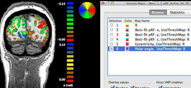
The sixth map "Polar angle" contains estimates of the location in polar coordinates; the calculated angle α is expressed relativ to the positive (right pointing) x axis and is simply obtained by applying the equation α = atan2(-y, x) at each voxel. Note that the sign of the value for the pRF y location is flipped (-y); this is done because the y axis in the implemented stimulus representation is defined from top (-) to bottom (+) while the coordinate system used in the unit circle of trigonometry runs from botton (-) to top (+). By flipping the y axis, the angles can be interpreted as in the unit circle, i.e. the angles are expressed with respect to the right half of the x axis (α = 0) and increase counter clockwise with α = 90 (π/2 radians) corresponding to the upper (-y) y axis, α = 180 (π radians) corresponding to the left half of the x axis and α = 270 (-π/2) is reached at the lower (+y) axis. In order to appropriately process (e.g. spatial smoothing) and visualize angle maps, the map type "a" has been introduced in BrainVoyager where angles are expressed in radians with positive values for the upper half of the unit circle and negative values for the lower half of the unit circle. The snapshot above indicates that the "Polar angle" map is represented as the special angle map type by the string "a [rad]" below the color bar. The positive and negative map maximum values "3.14" indicate (approximately) value π; furthermore, the color bar is also shown in a circular disk that helps to relate colors in the map to angles, which is especially helpful when using polar angle maps to separate early visual areas from each other.
As in conventional retinotopic mapping, the polar angle map (and to some extend the other maps) is very helpful to delineate early visual areas by observing horizontal and vertical meridian representations since they separate mirror-symmetric visual field representations in neighboring early visual areas. This is, however, best done on cortical surface representations. One way to proceed is to sample the volume maps on cortex mesh representations of the same subject. Another approach is to run the pRF estimation procedure directly on SRF-MTC data.
Note that eccentricity and polar angle maps are derived from the pRF x and y maps although in this example only bar stimuli were used and not the classical ring and wedge stimuli. While oriented bars at different locations prove to be an excellent stimulus for retinotopic mapping (e.g. Senden et al., 2014), it is possible to use or combine classical eccentricity and polar angle stimuli with bar-like (or other) stimuli in a single pRF experiment.
Copyright © 2023 Rainer Goebel. All rights reserved.