BrainVoyager v23.0
Measuring Cortical Thickness in Cortex Space
The major goal of cortical thickness measurements are group studies comparing cortical thickness values in various brain regions between different population samples. Cortical thickness group analyses require correspondence between regions in different subjects. Because cortex-based alignment matches marco-anatomical structures, such as gyri and sulci, it is an ideal approach to establish spatial correspondence for cortical thickness group analyses. While cortical thickness measurements are performed in volume space in individual brains, group analyses are performed in surface space in order to profit from cortical alignment. As described below, cortical thickness group analyses start with the measurement of cortical thickness on cortex meshes that have been produced in a preceding cortical alignment procedure. When cortical thickness surface maps (SMPs) are available for all subjects of all desired groups, computation of average thickness maps across subjects and group comparisons of thickness measurements in regions-of-interest can be performed. For each of these three steps, a separate tab is available in the Cortical Thickness Analysis dialog, the Measurement tab, the Group Maps tab and the POI Analysis tab. To launch this dialog, load a mesh and click the Cortical Thickness Analysis item in the Meshes menu.
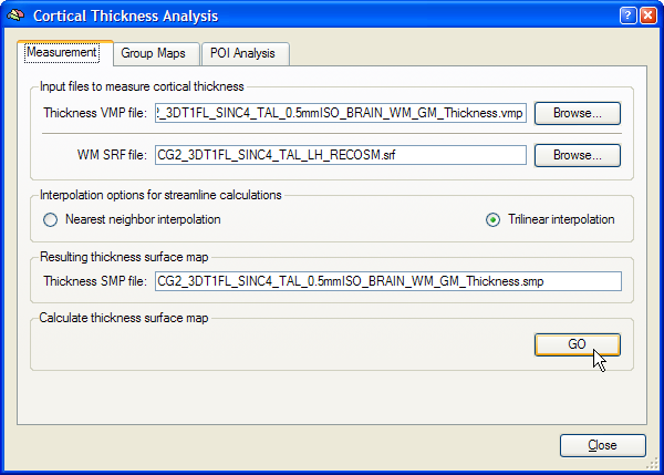
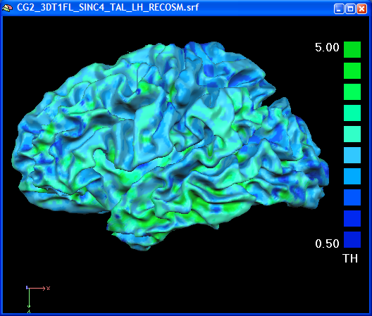
The name of the currently loaded mesh file is shown in the WM SRF file text box. This is typically a single hemisphere or a whole-cortex mesh file containing both the left and right hemisphere (after "merging" the two hemisphere meshes). If you want to choose another surface mesh, use the Browse button on the right side of the WM SRF file text box. To calculate the cortical thickness (streamlines) for each mesh vertex, the program needs as input the previously computed volume map containing the gradient component and thickness sub maps. If you have just computed or already loaded the volume thickness map, its name will appear in the Thickness VMP file text box. If this file is not available, use the Browse button on the right side of this text box to select the thickness VMP file. Make sure that the selected VMP file and the surface file are both from the same subject. The Interpolation options for streamline calculations field allows to select either the Nearest neighbor interpolation or Trilinear interpolation option (recommended) for the computation of streamlines. The output of the cortical thickness measurement will be saved in a surface map (SMP) file. A recommended name for this file appears in the Resulting thickness surface map text box matching the name of the thickness VMP file. To start the cortical thickness measurement, click the GO button in the Calculate thickness surface map field. After the streamline calculations have been completed, the cortical thickness surface map is shown superimposed on the mesh file (see figure below for an example). The SMP data structure resides in working memory but has been also saved to disk since it is used for subsequent group analyses.
Note that surfaces derived from different resolutions can be used to sample the high-resolution segmentation volume data. In the following snapshot, the standard "RECOSM" surface is used to calculate the surface cortical thickness map. For group analyses, you can use the standard surfaces coming from the cortical alignment procedure.
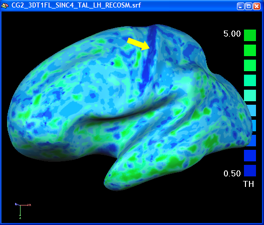
In the volume thickness map, the different thickness values in the anterior and posterior bank of the central sulcus was easily visible. In the folded state of a mesh, this is not readily seen. After overlaying the surface map on an inflated view of the brain, the thin posterior bank of the central sulcus is easily visible ("pops out", see figure below).
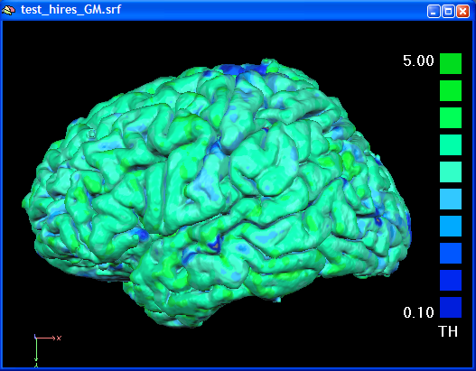
In the figure below the cortical tickness map has been computed using a GM / CSF boundary reconstructed from the high-resolution VMR data.
Copyright © 2023 Rainer Goebel. All rights reserved.