BrainVoyager v23.0
Intensity Histogram Analysis
In order to determine automatically a threshold separating white from grey matter, the intensity values of the data are analyzed in the step Find intensity peaks for grey and white matter.

More specifically a series of intensity histograms across several axial slices is computed (z = 54 + n*10, 0≤n<10). The 10 different histograms are drawn in different colors changing from blue (most superior slice) to red (most inferior slice). Intensity is on the X-axis (left side black voxels, right side white voxels) and the number of voxels per intensity (frequency) is shown on the Y-axis. The curves should show two major peaks, the first peak (left side) then corresponds to the intensity of grey matter whereas the second peak (right side) corresponds to the intensity of white matter. The program also shows a dialog showing the computed threshold value separating white from grey matter. This value is also shown as a vertical line in the intensity histogram. By using the Cut value spin box in the appearing dialog, the suggested value can be changed. It is recommended to change the cut value only in case that non-optimal segmentation results are observed. If the resulting WM-GM segmentation appears to have missed white matter regions, changing the value of the threshold slightly towards the grey matter peak might help to yield a better segmentation result. If on the other hand the segmentation result seems to have spread too much into grey matter, increasing the value slightly might improve the segmentation result. You may check different threshold values since the segmentation procedure (without bridge removal and cortex reconstruction and smoothing) lasts only about a minute to complete.
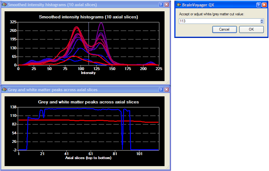
Note that the intensity values are only defined in the range 0 - 225. The reason for this is that intensity values larger 225 are reserved for specific purposes, such as indicating segmentation results in different colors.
Why not drawing just one intensity histogram pooled across all slices? The reason for drawing multiple slice-based histograms is to give information about the homogeneity of the intensity values across the slices. Axial slices were chosen because many sequences (i.e. MPRAGE) appear to have homogeneity problems along this direction. The white matter peaks of the different slices should be all lined up as shown in the graph above. If this is not the case, you should consider performing automatic inhomogeneity correction. The second graph also presents homogeneity information by tracing the white matter (blue) and grey matter (red) peaks across axial slices (54<z<171). If the blue line is horizontal within the x values 20 and 90, the data is homogeneous enough for the subsequent segmentation steps. The two diagrams remain on the screen after completion of the segmentation procedure. You may simply close these windows by clicking the respective Close icons.
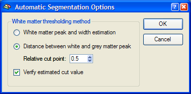
There are two methods implemented in BrainVoyager QX to determine the threshold value, the White matter peak and width estimation and the Distance between white and grey matter peak (default) method. The used method can be changed in the Automatic Segmentation Options dialog, which can be invoked by clicking the Options button in the Automatic Cortex Segmentation and Reconstruction dialog. The The peak-to-peak method is used as default and specifies the white-grey matter intensity threshold half way between the determined grey and white matter peak. The exact point is defined by the Relative cut point value (see snapshot above). This value is originally set to "0.5", which sets the WM-GM threshold exactly at the intensity value in the middle of the two peaks. If this value would be set to "1.0", the threshold would be set directly at the white matter peak, if it would be set to "0.0", the threshold would be set at the grey matter peak. You may change this value more towards the grey or white matter peak in case you find a systematic error with your data sets when using the default value. Note that you can change the threshold value also during the segmentation process as described above. The respective dialog is only shown if the Verify estimated cut value option is turned on (default).
The white matter peak and width estimation method has been introduced as a second method because the peak-to-peak method did not always produce robust results across different scanners and MR sequences. The main problem is that it is only dependent on the distance between the grey and white matter peaks but does not take into account the width of the distribution around the peaks. This may lead to results where the segmentation is too much biased towards white or grey matter intensities. The white matter estimation method starts with the white matter peak and determines the intensity distribution on the right side of that peak. More specifically, the value on the right side is determined at which the corresponding frequency drops below 10 percent as compared to the frequency at the WM peak. This procedure estimates the width of the white matter distribution. The histogram analysis is only performed on the right side of the WM peak because on the left side the white matter and grey matter distributions are overlapping to a certain degree.
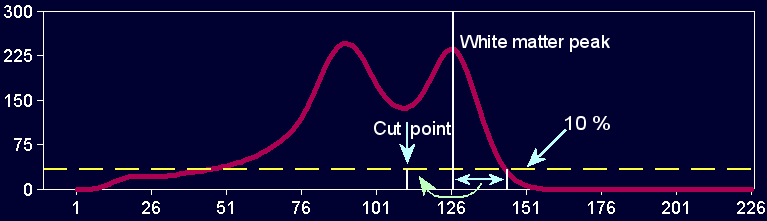
The estimated threshold value is finally determined by subtracting the distance of the 10 percent intensity value to the WM peak from the WM peak (mirroring of the distance on the right side to the left side, see graph above).
Copyright © 2023 Rainer Goebel. All rights reserved.