BrainVoyager v23.0
Group Alignment
Two Group Alignment Approaches
Pairwise CBA of multiple sources to specified target. While the pairwise alignment CBA described in the previous topic can be used to align cortical hemispheres from multiple subjects to the same target brain, it requires manual interactions to select and start the alignment for the varous curvature smoothing levels of each source-target alignment pair. These manual steps can be avoided by using the group alignment possibilities available in the Align Group tab of the Cortex-Based Alignment dialog. In this tab a set of source hemispheres can be added to a hemisphere curvature list. When running the group alignment, each of the included source hemisphere curvature maps will then be pairwise aligned in turn to a specified target hemisphere curvature map. In order to ensure that the pairwise group alignment approach will be used, the Align each entry to target sphere option need to be selected in the Alignment mode field.
CBA of multiple sources to dynamically generated group average target. While the pairwise group alignment mode allows to avoid manual interactions, it requires selection of an individual cortex mesh as the target brain and alignment results might be influenced by that choice. BrainVoyager offers also a version of CBA that circumvents this issue operating on a group of hemisphere meshes without the neeed to specify a target brain. In this moving target group averarging approach, the target brain is calculated and updated automatically during the alignment process. More specifically, the target curvature is computed repeatedly during the alignment process as the average curvature across all hemispheres at a given state of alignment. Like the pairwise alignment, the procedure starts with the most coarse curvature maps and proceeds to increasingly fine-grained curvature maps. At the begin of a new curvature smoothing level as well as several times within an alignment stage, the curvature maps are averaged using the obtained alignment result at this moment. The updated group average curvature serves as the new alignment target for a specified number of iterations before the curvature is averaged again. Since the target curvature thus changes over time, it is referred to as a "moving target". This process is repeated until the most fine-grained curvature maps have been processed. The target hemisphre is thus not selected a priori but emerges and refines during the process. The final result at the end of this approach thus consists of a created group target curvature map as well as the alignment of all individual hemispheres to that new target. In order to to use the moving target group averaging approach, the Align to dynamic group average option in the Alignment mode field need to be selected, which is the default setting. Note that the list of curvature hemispheres will be filled slightly differently in the two alignment approaches: In the moving target group averaging approach all hemispheres need to be added to the curvature hemispheres list while in the group pairwise alignment approach, all but one source hemispheres will be included (one hemisphere is used as target) except the target hemisphere is selected from an external (e.g. atlas) brain.
While it is recommended to use the dynamic group averaging approach (default), the pairwise alignment usually leads to similar results and it is the only possibility in case one explicitly wants to align all group hemispheres to a specific external (atlas) target brain.
Preparing Group CBA
Group Curvature List
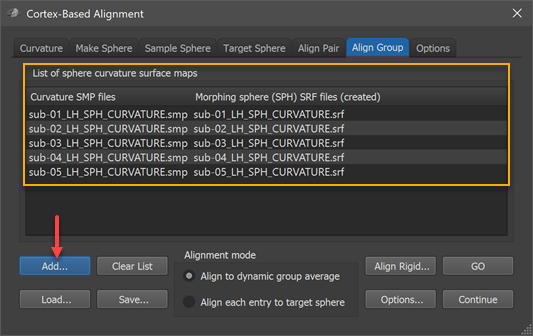
The group-CBA process aligns the curvature maps provided in the group curvature list in the List of sphere curvatrue surface maps field of the Align Group tab (see screenshot below). In order to add the curvature map of a participant, the Add button can be used (see arrow in screenshot below), which will launch a file selection dialog. The selected curvature SMP file (e.g. "sub-01_LH_SPH_CURVATURE.smp") will appear in the left column of the group curvature list while the right column shows the name of a standard sphere that will be created at the begin of group-CBA for the respective subject; the name of the mesh will be based on the name of the selected curvature map (e.g. "sub-01_LH_SPH_CURVATURE.srf" in the example). During CBA, the subject's sphere meshes will be saved regularly to keep the perfomed vertex movements for each hemisphere over time during the alignemnt (morphing) prcess. The screenshot below shows the group curvature list after the left hemisphere curvature maps of 5 subjects have been added. Note that all selected curvature maps need to represent the same hemisphere; in order to align both hemispheres of a group of subjects, the alignment must be run twice, once for the left ("LH") and once for the right ("RH") hemispheres.
The moving target group averaging CBA approach can now be started by clicking the GO button in case that the Align to dynamic group average option is selected in the Alignment mode field (default). When selecting the Align each entry to target sphereoption in the Alignment mode field, an explicit target has to be defined in the Target Sphere tab before the CBA process can be started (for details see pairwise alignment topic). In case that the target curvature (provided as a spherical PMP map) is coming from one of the group members, the respective curvature map should not be included in the group curvature list. For reproducibility and later reuse, the filled curvature map can be saved as a group alignment list (GAL) text file (e.g. "Group_LH_N-5.gal") to disk using the Save button. A group alignment list file can be reloaded using the Load button while a (partial) list can be cleared using the Clear List button.
Alignment Parameters
The coarse-to-fine CBA process is controlled by various parameters that are carefully adjusted to usually produce very good results. It is however possible to adjust the parameters, if desired, in the Cortex-Based Group Alignment Parameters dialog that can be invoked by clicking the Options button in the Align Group tab (see screenshot below).
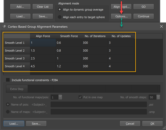
The group alignment parameters table (orange rectangle) in that dialog holds the (default) settings that are used during the alignment procedure. While the table rows are sorted (top to bottom) from most fine-grained (Smooth Level 1) to most coarse (Smooth Level 4) curvatrue map, the alignment process starts with smooth level 4 and progresses to smooth level 1 in a coarse-to-fine fashion. The four columns of the table contain, for each smoothing level curvature map, the CBA parameters used during on-sphere morphing. The values in the Align Force column determine the force used by each vertex to follow the local curvature gradient minimizing curvature differences between the source and target curvature map. These values should not be set to very high values since this might destabilize the process introducing vertex "foldings". If the alignment force is not set too high relative to the smoothing force in the Smooth Force column, topographical issues are avoided. The No. of Iterations column specifies how many iterations should be performed with the respective parameters at each smoothing level. The values in the No. of Updates column are only used for the dynamic group averaging approach, i.e. they are ignored when running the explicit target pairwise group CBA. In the dynamic group averaging (moving target) approach, a new group average curvature map is created as many times as specified in this column based on the achieved alignment at that point. When using the default values, a new group map is calculated 4 times for the two coarsest smoothing levels while 3 new group maps are calculated for the two more fine-grained levels. A new group averaging map is always calculated at the begin of each smoothing level followed by (#updates - 1) further updates during alignment at that level; with, for example, 300 iterations and 4 updates, a new group average map will be calculated before the morphing starts (iteration 0), and after iterations 75, 150 and 225.
Note. The group alignment parameters are reset when restarting BrainVoyager. You can, however, save custom alignment values to disk as GAP files (files with extension '.gap') using the Save button in the Cortex-Based Group Alignment Parameters dialog and load them in subsequent sessions using the Load button. GAP Files with the default values for versions 22 and 23 of BrainVoyager are provided.
Optional Pre-Step: Rigid Sphere Alignment
While CBA usually enhances correspondence without explicit specification of landmarks, it is important to start CBA at a stage where sulci and gyri are already relatively close to each other on the sphere so that the gyri and sulci of the maximally smoothed curvature maps overlap to some extent. In case that major gyri and sulci of hemisphere meshes from different brains deviate very much from each other (despite initial ACPC, MNI or Talairach normalization) sub-optimal alignment results could be obtained. In order to reduce the likelihood of partial mis-alignments, BrainVoyager offers the possibility to run a rigid sphere alignment step prior to the locally operating main process. In this "rigid" alignment step, all included source spheres are rotated around the center using a combination of values for each axis in a specified range. The range of values for the 3 axes can be specified in the Rotation ranges field (default -20 to +20 degrees for X and Y axis, -10 to +10 degrees for Z axis). The respective No. of steps values define the granularity of steps in the specified range, ie. together the range and the number of steps define the density of the performed parameter grid searrch. For each combination of tested rotation values, the global curvature alignment error with respect to the target curvature map is recorded and shown in the Log during processing. The parameter set producing the best fit (smallest curvature alignment errror) for each hemisphere will be selected and stored in a rigid group alignment (RGA) text file. At the begin of subsequent CBA (i.e. after clicking the GO button in the Align Group tab) the RGA file will be read from disk and the rotation values stored for each subject's hemisphere will be applied to the standard sphere meshes that will be created at the begin of the actual group CBA procedure. After the rigid alignment step the subsequent CBA will begin at a better starting point, which often leads to better results than when not using this step.
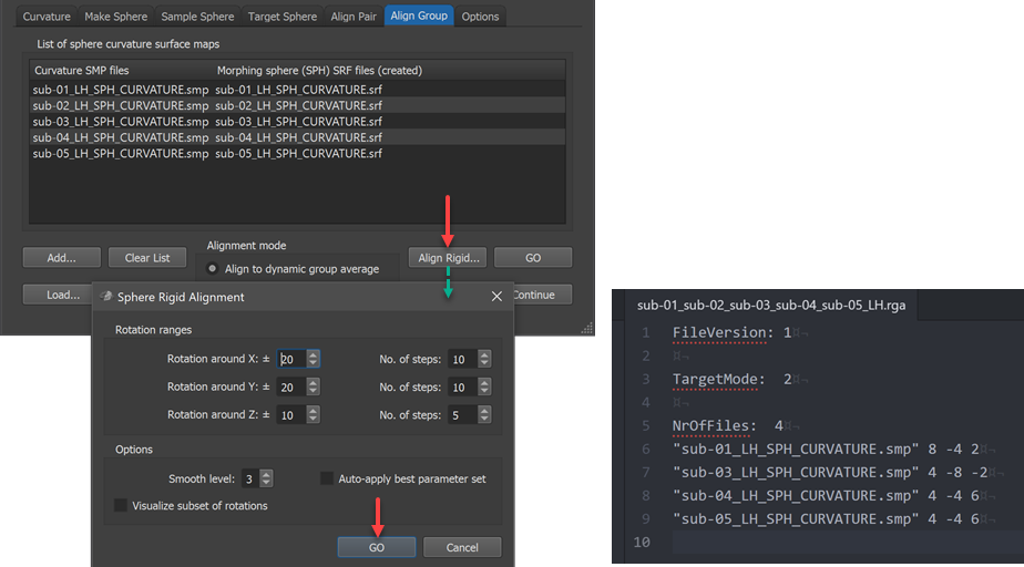
Note that the Auto apply best parameter set option in the Sphere Rigid Alignment dialog should not be turned on (off by default) since the calculated rigid alignment parameters will be automatically applied when starting group alignment (this is different for the manual pairwise alignment process). When rerunning CBA with the same hemisphere curvature files (but potentially different parameters), rigid sphere alignment need not to be executed again since CBA will look for a matching RGA file on disk, which, if found, is used automatically. In case one wants to rerun CBA with the same files but one wants not to perform rigid sphere alignment, the RGA file needs to be manually removed (or renamed) in the respective directory on disk. The generated RGA file name will contain the individual subject ID's in case one uses 10 or less files and it will have a generic name when using more than 10 subjects. In the example case shown in the dialog above, the generated RGA file is stored with the name "sub-01_sub-02_sub-03_sub-04_sub-05_LH.rga" for dynmic group alignment. For the pairwise explicit target approach with subjects 1, 3, 4 and 5 aligned to subject 2, the generated RGA file name is "sub-01_sub-03_sub-04_sub-05_Target_sub-02_LH.rga". If more than 10 files are involved, a generic name "Group_N-[n-files]_[LH|RH].rga" or "Group_N-[n-files]_Target_[ID]_[LH|RH].rga" would be generated. The scrrenshot above shows on the lower right side the generated .rga file for the example data. Note that while the file name lists 5 subjects, there are only 4 files listed in the file; the reason is that the hemisphere curvature map of the 2nd subject has been specified as the rigid alignment target and it is thus dropped from the list.
Note. While not necessary for the actual CBA, a target brain needs to be selected in the Target Sphere tab also when subsequently using the dynamic group averaging approach, which can be a curvature map of one of the included hemispheres as well as an external (atlas) hemiphere. The specified target curvature is only used for the rigid sphere alignment step but not for the subsequent dynamic group averaging CBA. If rigid sphere alignment is not used, specification of a target hemisphre is not needed.
Running Group CBA
If all preparations have been completed, the vertex-morphing CBA process can be started by clicking the GO button in the Align Group tab of the Cortex-Based Alignment dialog. In case that the pairwise explict target approach is used, each source sphere will be loaded and the subjects' curvature map will be aligned to the selected target curvature map using all curvature maps in a coarse-to-fine approach. Only if the alignment of a source hemisphere has been completed, the program moves to the next hemisphere. This is different when the dynamic group averaging (implicit target) approach is used. In this case, the program aligns only a few iterations for one source sphere before going to the next. If all spheres have been somewhat aligned to the current group average curvature, a new group average will be computed, which should be a better target than the first one because each source mesh has been aligned towards the (previous) averaged curvature map. Now another run through all source spheres is perfromed where each source sphere aligns somehat towards the target. With the improved alignment, another new group average map is calculated and so on. The process continues until all smoothing levels have been used. During the process, the program shows the frequent switches between source brains that are only aligned for a short amount of time to the current target brain. The alignment quality can be assessed by observing the displayed curvature overlay colors that are described in the previous topic ("good" colors: pink = overlap of concave curvature ("sulci on sulci"), yellow = overlap of convex curvature ("gyri on gyri"); "bad" colors: blue = overlap of convex and concave ("sulci" on "gyri"), orange = overlap of concave and convex ("gyri" on "sulci").
Main Result - Sphere-To-Sphere Mapping (SSM) Files
After the alignment process has completed, the morphed (aligned) spheres are sampled from a generic standard sphere resulting in a sphere-to-sphere mapping (SSM) file for each subject describing the displacement of each vertex (e.g. "SUB-01_LH_SPH_GROUPALIGNED.ssm" for the first subject in the example, see figure below). The created SSM files allow to bring information from the source hemisphere (e.g. statistical maps, time courses, vertex coordinates of folded sphere mesh) into corresponding locations of the group (target) hemisphere. The SSM files from each source brain will thus be transformed into a common target space, which will correspond to a selected target brain when using the pairwise group alignment or a representative group brain when using the dynamic group averaging approach. For some applications, also the inverse transformation of information is needed, i.e. when one wants to transfer a parcellation scheme from an atlas brain to a source brain. For this purpose, the program will also save a .SSM file ending in the substring "_inv.ssm" (e.g. "SUB-01_LH_SPH_GROUPALIGNED_INV.ssm" in the figure below).
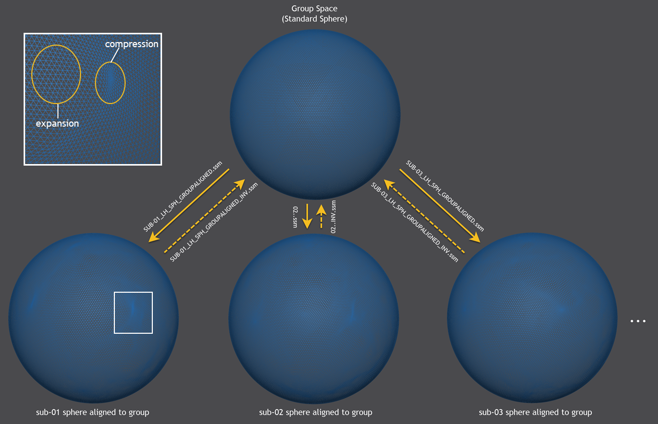
The figure above shows in the lower half the morphed (aligned) hemisphere meshes of the first 3 subjects that are sampled by the generic standard sphere shown at the top producing the .SSM output files shown next to the sampling arrows in the middle part. While the generic group mesh is a sphere with regular vertex spacing, the subject-specific spheres exhibit non-linear local transformations such as expansions and compressions. For a section (white rectangle) of the morphed sphere of subject 1, examples of such non-linear effects are shown enlarged in the upper left part of the figure.
Visualization of Group Results
As a convenience, the created SSM files are used to prepare various files to visualize the alignment results of the group data. These files are usually stored in the parent directory of the individual curvature maps. The most relevant stored files are:
- GroupAlignedCurvatureMaps_LH_N-5.smp - the aligned curvature maps (see below)
- GroupAlignedCurvatureMaps_LH_N-5.srf - a standard sphere named in the same way as the curvature SMP file
- GroupAlignedAveragedFoldedCortex_LH_N-5.srf - the folded group brain resulting from averaging aligned vertex positions
- GroupCurvatureList_LH_N-5.cal - a curvature averaging list (CAL) text file
- GroupShapeList_LH_N-5.sal - a shape averaging list (SAL) text file
The "N-[n-files]" substring will be adjusted accordingly, i.e. it is "N-5" in the example since 5 curvature maps have been aligned. Note that all stored files can also be created manually by using the average curvature and average shape functionality in the Options tab of the Cortex-Based Alignment dialog (see next topic). The easiest way to visualize the aligned curvature maps would be to load either the sphere (GroupAlignedCurvatureMaps_LH_N-5.srf) or the folded mesh (GroupAlignedAveragedFoldedCortex_LH_N-5.srf) followed by loading the aligned curvature maps (GroupAlignedCurvatureMaps_LH_N-5.smp).
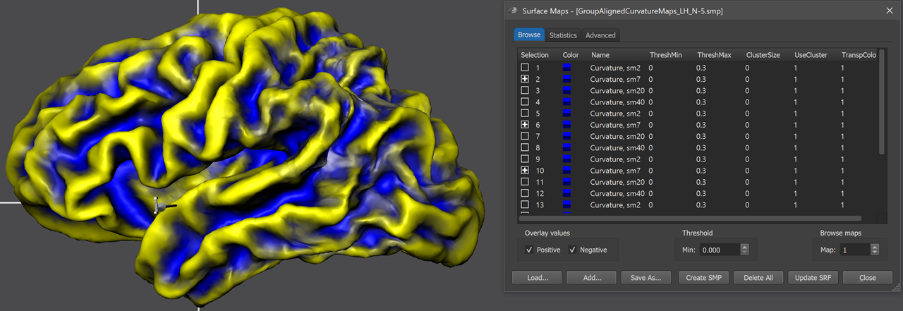
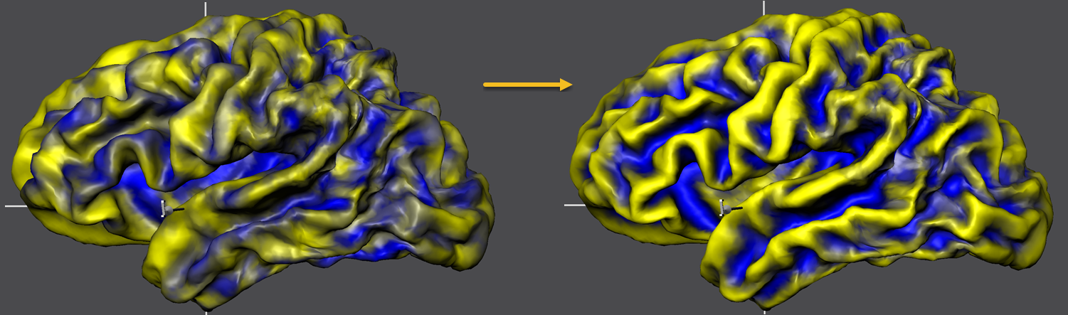
At the end of group-CBA, the program automatically displays the aligned surface maps allowing to visually judge final alignment quality. The curvature maps are either overlaid on a standard sphere or on a created folded group hemisphere. The screenshot above shows the folded group brain with the overlaid curvature maps of the 5 included subjects of the example data. When opening the Surface Maps dialog (right side above), the curvature maps of all included subjects are shown from top to botton with all 4 smoothing-level variants. The program has automatically selected the second map from the 4 maps of each subject. Note that the individual curvature maps have been added after SMP alignment, otherwise the CBA improvement of curvature overlap would not be displayed but the state before alignment. For comparison, one can simply overlay the non-aligned curvature maps by loading (adding) them from disk and selecting the same smoothing level for all subjects as for the aligned curvature maps. For the example data, the figure below shows the unaligned curvature map overlay on the left side and the aligned curvature map overlay on the right side indicating a substantial improvement of achieved across-hemipshere alignment.
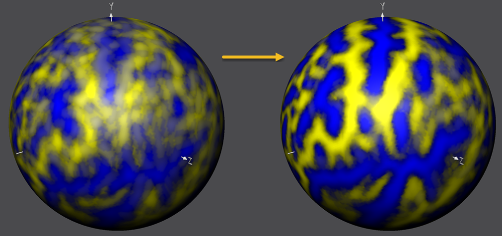
The figure below compares the unaligned and aligned curvature maps in the same way but overlaid on the standard sphere serving as the common target group space. The substantial improvement in curvature overlap achieved by CBA is apprarent in both visualizations. The next topic will describe how to calculate and compare further visualizations of the achieved group results including curvature and shape averaging, creation of probabilistic maps and displaying information about the time course of alignment.
With the completed group-CBA, the created SSM files can now be used for subsequent applications such as running statistical group analyses in aligned space, aligning patches-of-interest and aligning other (non-curvature) surface maps. It is also possible to create probabilistic maps and maximum probability maps that are useful for building a custom brain atlas. One may also consider to run more advanced versions of CBA that include alignment of anatomical landmarks or functional areas as additional alignment sources.
Copyright © 2023 Rainer Goebel. All rights reserved.