BrainVoyager v23.0
EEG / MEG Source Imaging and Analysis
Source reconstruction allows projecting averaged channel time-courses (ACT) and single-trial data sets (STD) to all vertices of a mesh source space, and this is normally done for each separate protocol condition after channel data preparation and preprocessing. Although it is possible to edit protocols, prepare design matrices and combine MTCs in single-study (SS-) and multi-study (MS-) GLM (fixed- or random-effects) analyses, similar to fMRI cortex-based analyses, a more direct and powerful alternative approach for ERP/ERSP cortical source imaging and analysis, that does not require protocol editing and GLM design matrix building, but still allows generating EEG and MEG source images as well as plots from the combination of many channel data sets with their corresponding inverse solutions for specified target and baseline time or time-frequency intervals is available in BrainVoyager QX in the 6th tab of the EMEG Suite dialog.
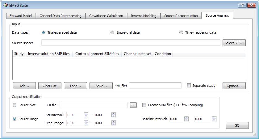
Similar to EEG/MEG source reconstruction, it is necessary to specify the input data type and the output options. But there are three supported types: trial-averaged time-courses or spectral power (ACT), single-trial data (STD) and time-frequency data (TFD), and, for each of these, two output options: source imaging (default) and source plotting. When starting from trial-averaged channel time-courses (ACT files) and working in source image mode, this tool generates a series of maps, one per each single latency within the selected interval of interest, called Target ("For") Interval. With the help of the Movie Studio tool, it is then possible to build up a full activation movie for the ERP/ERF responses to a given condition. When starting from single-trial channel data (STD files) and time-frequency data (TFD files), and working in source image mode, this tool allows generating parametric statistical maps via t-tests at each virtual electrode (point source), thus mapping the main and differential effects of the ERP/ERSP responses, averaged across the target interval time and frequency points and in comparison to a baseline interval. Statistical maps of differential effects will only be generated when two experimental conditions or two groups of subjects are present in the prepared list of files prepared (EMEG list, see next paragraph).
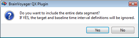
Note: Before starting the user is asked about whether or not using the entire data segment for the source imaging and analysis, thereby the target and baseline interval definitions would be ignored. If responding "yes", only the first trial of the data set will be considered with no averaging and no baseline normalization of the projected data. This choice is particularly adviced when ACT and TFD data were obtained from a single unique data segment (see section on channel data preparation and preprocessing for more details). In this case, no trial averaging is performed (because there is just one trial included in the calculations) and no baseline normalization is used (because a single continous data segment is considered).
Source Analysis Design Preparation
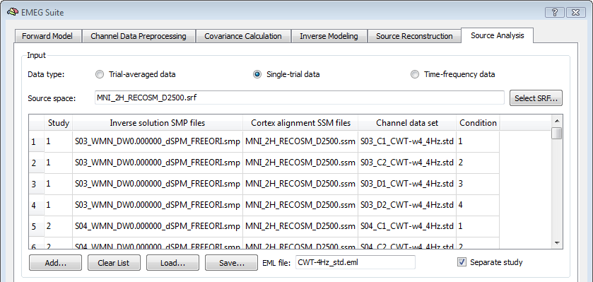
In order to implement this kind of "summary" distributed source analysis, we need a valid inverse solution (SMP) for each data set we want to combine in the source analysis. In the list of EEG/MEG data sets (EML), besides the inverse solution to apply and the name of the channel data file, a progressive index for the study (i.e. group, subject, session, etc...) and for the condition to which each data set belongs has to be specified. Then, the data projection will be performed in "batch" for all data sets on the current mesh (which is therefore implicitly used as the common source space). Since we can use a common source space even for multiple subjects, we always need a sphere-to-sphere mapping (SSM) file in this list that will establish the right correspondences from any original sphere to the current (target) sphere.
Note: In the absence of a "real" SSM (i.e. if we have not performed cortex-based alignment), we can use an "identity" SSM file for the current SRF used as source space. Such an SSM file is written to disk whenever a source reconstruction on this mesh is performed for any data set via the functions of tab 5th, meaning that all data sets are projected to the same source space via the same sphere (of course to get this SSM it is enought to do the reconstruction once for the current mesh).
In order to successfully prepare the final source analysis, it is important to consistently identify and label the different studies and conditions of the analysis. By default, adding a new entry to the EML list corresponds to adding a new condition of a given session or subject. The term study can therefore either refer to a single session or to a single subject (with multiple conditions); one or more conditions can be pooled across different studies (forming a session or a group) if and only if all studies are present for that condition. An EML list will not be accepted if one condition is not present in all studies. If the "Separate Study" option is checked, the conditions will be not pooled across studies and different images or plots will be generated for different each study separately. For instance, the "Separate Study" option is to be checked if individual condition-specific subject images are to be generated for a second-level (random effects) analsyis within the general ANCOVA framework.
Important: After preparation, the EML file should be always saved and in such a way to appear with the new given name in the appropriate field ("EML File:"). If not saved (and/or reloaded) explicitly, the program will not use the current list but eventually starts with the last EMEG list in memory (which is an empty list if the analysis is operated for the first time).
In source image mode, after defining the target interval of activity (e.g. from 0 ms to 200 ms) and the baseline interval (e.g. from -200 ms to 0 ms) with respect to the trial trigger, the analysis is launched by clicking the "GO" button. Upon completion a set of SMP files will be saved in the current folder containing all the computed maps. In time-frequency input modality (TFD), a frequency interval (e.g. from 15 Hz to 30 Hz) is also to be specified. In source plot mode, a list of regions of interest should be loaded in the appropriate field as a POI file and new summary data sets will be created for the corresponding regional sources.
Source Imaging
When working on trial-averaged channel time-courses (ACT files) and in source image mode, a new SMP will generated for each condition containing a series of surface maps with the projected ERP/ERF activity at each single latency of the target interval. If more studies are added to the same list the source data are averaged within the same condition, unless the separate study option is checked. By launching the "Overlay Surface Maps ..." dialog from the Meshes menu, the Surface Maps dialog appears with all maps, as shown in the figure below:
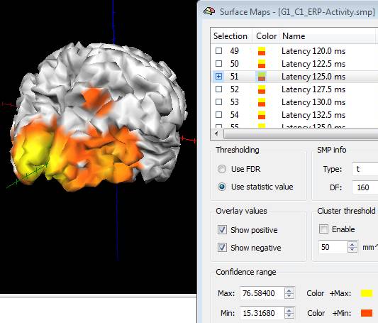
Note: the maps generated from ACT are only "descriptive" of the EEG/MEG source activity distribution and have no statistical significance. In fact, each map contains the projection of channel ERP/ERF at one target latency to the current mesh after subtraction of the baseline (mean of the baseline interval) and after re-scaling between 10% and 100% of the entire spatial distribution.
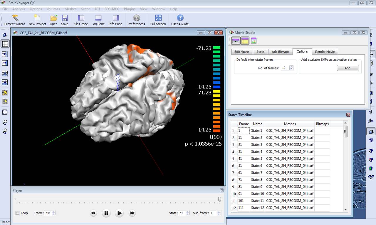
The series of maps in the SMP can be converted to a BrainVoyager movie (BMV) for easy frame scrolling along a virtual time point axis. Just close the Overlay SMP dialog, invoke the Movie Studio tool from the menu Scene -> Movie Studio ..., deselect the options of keeping the viewpoint and mesh slice levels, and "Add" all maps to the frame list as activation states. Once the frame list is complete, it is possible to use the movie player to visualize the movie in the surface module, as shown in the figure below:
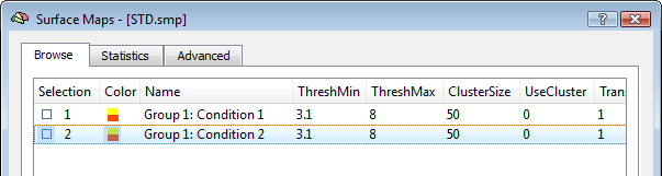
The activation movie is a very convenient tool for visual evaluation of the EEG/MEG activity. However, the movie is based on the projection of pre-averaged channel data and, therefore, it is not possible to evaluate "statistically" the difference between two intervals or between the two experimental conditions in a certain interval of latencies. To do so, single-trial and time-frequency data sets are to be used. In this way, each single-trial time-course is projected and the average source power in target and baseline intervals are considered for a statistical evaluation at each single virtual channel. At the end of the calculations, new SMP files will be written in the current folder containing main and differential effect statistical maps for the pooled data sets. The output SMPs containing the source images generated from single-trial and time-frequency data sets (STD/TFD) will be different depending on whether the "separate study" option is checked or not. When this option is not checked, each single statistical map expressing the main effects of a given condition or the differential effects between two conditions will be obtained after pooling (concatenating) all study trials belonging to the same condition (fixed-effects analysis). This way, the number of output SMPs will be equal to the number of conditions and stored to separate SMP file. An additional SMP file will be created for differential effects when two conditions are present in the design, as shown in the figure below.
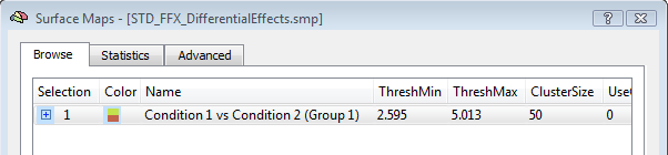
Note: The term "Group" in the SMP names (again) refers to either multiple sessions of the same subjects (submitted as separate studies) or multiple subjects of the same group. Of course, it' s up to user the decision of how data sets should be pooled in the final source statistics.
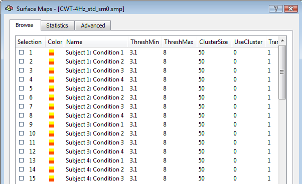
When the "separate study" option is checked, each single study is interpreted as a "subject" and condition-specific trials are not pooled. Moreover, the generated subject- and conditin- source images are standardized as z-score maps. One unique SMP file will be finally generated with all standardized images from all subjects and conditions, ready for the ANCOVA framework as in the example below.
Source Plotting
In source plot mode, a series of regions of interest as As a result, new EEG/MEG data files will be written in the current folder that will refer not the original channel configuration, but to new "regional" sources. Separate files will be generated for separate regions, experimental conditions and groups of subjects. When starting from ACT or STD, a new ACT file will be generated contaning the average source power time-course. When starting from a TFD, a new TFD file will be generated contaning the average source power time-frequency response.
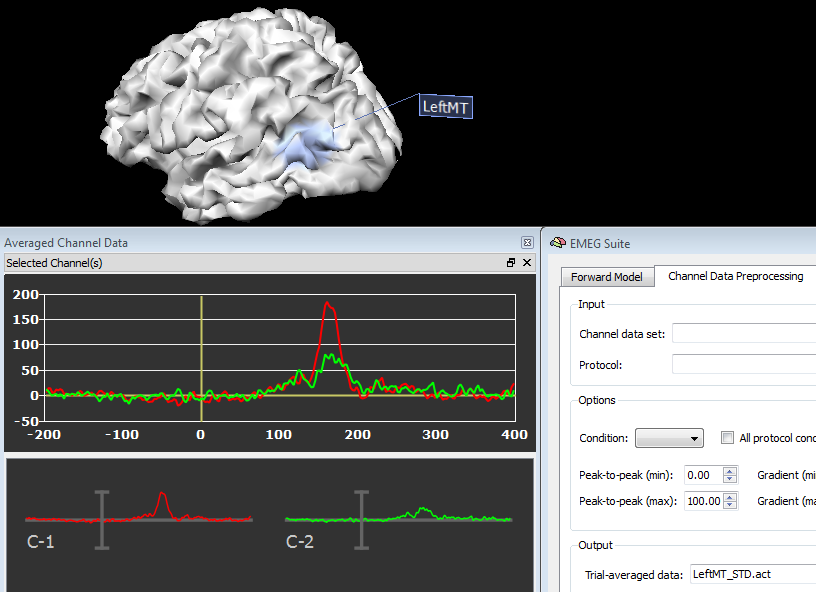
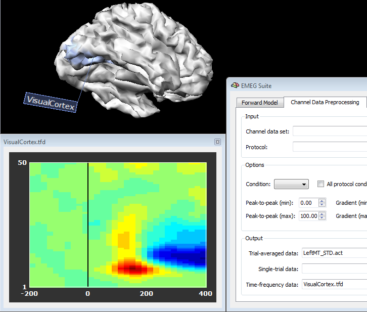
In order to plot the new source data, just switch back to the Channel Preprocessing Data (2nd tab) and select the appropriate files in the appropriate fields. In fact, source plots will be generated from the regions as these were standard channels, as shown in the figures below, respectively for a source ACT or TFD file:
Copyright © 2023 Fabrizio Esposito and Rainer Goebel. All rights reserved.