BrainVoyager v23.0
Mirror Representations and Field Sign Maps
In order to delineate early visual areas, polar angle maps (or at least mapping of the horizontal and vertical meridians) are required. Polar angle maps show relatively smooth transitions in the color coding representing adjacent angles of a checkerboard wedge (see inset in figure below). Since early visual areas border each other with a mirrored representation of the visual field at the horizontal and vertical meridians, the area boundaries can be specified at the "turning points" of the colour codes. As an example consider the dorsal region in the figure below where colors are based on the standard BrainVoyager QX overlay LUT after a cross-correlation analysis. The yellow (and green) colour along the cut represent the horizontal meridian of the left lower visual field. Moving anteriorly, the colours change from yellow to red and then back to yellow. The red turning point represents the vertical meridian separating dorsal area V1 from dorsal area V2 (mirror representation). Moving further anteriorly, the colors change to yellow and then back again towards red. The yellow turning point represents the horizontal meridian separating dorsal area V2 from dorsal area V3. Moving further anteriorly, the next red turning point separates dorsal area V3 from area V3a. Note, that in this region there are also blue and green colours indicating that V3A also represents the upper left visual field (c.f. Tootell et al., 1997). The colours in the ventral part of the flat map represent the left upper visual field. As in the dorsal region (although not as clear), colour turning points represent the horizontal (green) and vertical (blue) meridians. The first blue turning point marks the transition from ventral V1 to ventral V2. The next green turning point demarcate ventral V2 from VP. Finally, the most anterior blue turning point demarcates VP from ventral V4 (V4v).
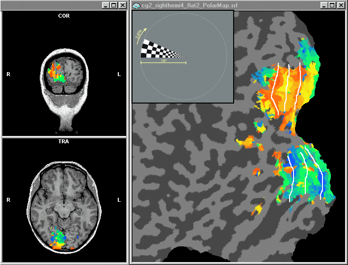
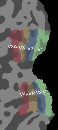
Note that in the figure above, a cross-correlation analysis was computed not for the full visual field (360 degrees) but only for the left half of the visual field (radiological convention is used). This improves the quality of the mapping result since no impact from the other half of the visual field is considered (which actually does occur more and more strongly if one moves higher in the visual hierarchy) and all available 20 colors are used for one hemisphere. In the recent releases of BrainVoyager (version 3.9 and above), special cross-correlation files for analyzing mapping data are distributed (EccenCrosscorr.rtc, PolarRightHemi.rtc, PolarLeftHemi.rtc) together with appropriate protocol files (Eccentricity.prt, Polar.prt). These files assume that one complete stimulation cycle (i.e. one rotation of 360 degrees) lasted exactly 32 measurements. Since this number might be different in your experiments, you have to adapt the example files to your needs. Using a polar mapping result as described, you can demarcate manually the boundaries between early visual areas using an external graphics program as was done in the figure above (white lines). You can also use Brainvoyager's surface drawing tools to delineate area boundaries. Invoke the Region Deletion and Coloring Options dialog by clicking the Floodfill options... menu item in the Meshes menu. In the dialog, check the Coloring mode option and select a color index in the Fill index text box for drawing, i.e. color index 1 for area V1, color index 2 for area V2 etc. You can change the RGB color values of the color indices and save them to disk using the local file menu. Note that each color index defines two color values, one is used for coloring convex and one for cancave regions. The figure below shows the result of interactively defining early visual area boundaries.
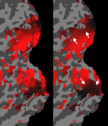
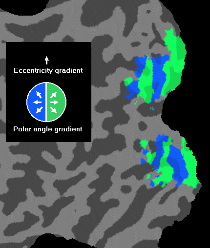
The computation of field sign maps (Sereno et al., 199?) is a more objective method for delineating early visual areas requiring both a polar angle and an eccentricity mapping experiment. If the mapping data is of good quality, this method works well for delineating V1 to V3/VP but it does not produce good results for higher areas which represent more than one quadrant of the visual field. Field sign maps exploit two properties of early visual areas. First, eccentricity roughly increases in the same direction across all early visual areas representing the same quadrant of the visual field. The direction of increase can be computed locally and specifies an eccentricity gradient. In the figure below the gradient directions are shown for some locations with a white arrow.
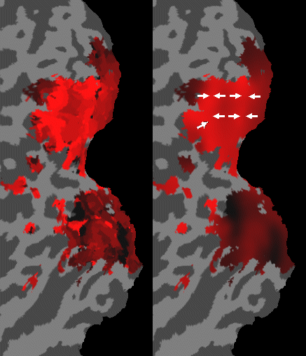
A second feature of the visual system exploited in the computation of field sign maps is that early visual areas border each other in a mirrored representation. Polar angle maps reflect this as described above. If one computes locally polar angle gradients, the horizontal and vertical meridians are detectable at those locations where the gradients maximally change their direction. This can be seen in the figure below where some polar angle gradients are shown.
A second feature of the visual system exploited in the computation of field sign maps is that early visual areas border each other in a mirrored representation. Polar angle maps reflect this as described above. If one computes locally polar angle gradients, the horizontal and vertical meridians are detectable at those locations where the gradients maximally change their direction. This can be seen in the figure below where some polar angle gradients are shown.
The combined analysis of the two gradient maps (eccentricity and polar) allows to locally assign whether an early visual area contains a mirror or a non-mirror representation of a respective visual field quadrant. In this analysis the angle between the polar angle gradient and the eccentricity gradient are computed at each vertex of the surface. If this angle is below 180 degrees, the location is assigned as "mirrored"; if the angle is above 180 degrees, the location is assigned as "non-mirrored". This attribution of "field sign" is visualized in the inset of the figure below. If a location is assigned as mirrored it receives color 1 (i.e. green), if it is assingned as non-mirrored it receives color 2 (i.e. blue).
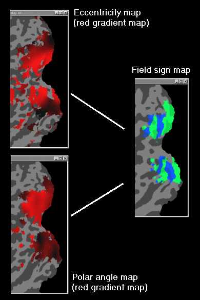
Since the assignment of field sign is a local computation, it is vulnerable to noise in the data. It is therefore recommended to smooth the data to some extent. To get a good local estimate of the eccentricity and polar angle gradient, the different colors of the respective maps are first converted to different brightness values of a single color. With the recent BrainVoyager distributions (version 3.9 and above), special overlay LUT files are included for this purpose (EccenRedGradient.olt, PolarRightHemiRedGradient.olt, PolarLeftHemiRedGradient.olt). Load the respective file after you have clicked the Read func button in the Mesh Morphing and Coloring dialog (you can load the .OLT file, of course, already when you compute or load the cross-correlation result within the .VMR project). The result on the flat map should now look similar as the ones shown in the red colored eccentricity and polar maps on the left side of the respective figures above. To smooth the map, we recommend to apply LUT smoothing once and then 10 times RGB smoothing (an explanation of the two types of smoothing can be found in topic Volume- and surface-based analysis of retionotopic mapping experiments). The result on the flat map should now look similar as the ones shown in the red colored eccentricity and polar maps on the right side of the respective figures above. You should save the resulting maps to disk (i.e. nn_rh_flat_EccenRedGrating.srf, nn_rh_flat_PolarRedGrating.srf). To compute the field sign map, BrainVoyager now requires that the eccentricity mapping result has been loaded and that a link to the polar mapping result is established using the Use information from file option in the Mesh Morphing and Coloring dialog. Now you can click the Field sign map button in this dialog which should result in a map as shown in the figure above.
The figure below summarizes the required information for computation of field sign maps: Smoothed red gradient map of the eccentricity mapping result (loaded) and smoothed red gradient map of the polar mapping result (linked). Based on these two pieces of information, the field sign map is computed (right side in figure below).
Note. The local neighborhood used in field sign assignment as well as in LUT smoothing is controlled with the Nr of nbr iterations value in the Morphing and Coloring Options dialog. This value is preset to 3 which means that up to the third level of direct neighbor voxels are considered (value 1 = all direct neighbors, value 2 = all direct neighbors plus their direct neighbors and so on). To gain a feeling of the influence of this value on the computation of field sign maps, you should recompute the maps using values in the range from 2 to 10.
Copyright © 2023 Rainer Goebel. All rights reserved.