BrainVoyager v23.0
Creating pRF Model Time Courses
Since the subsequent pRF estimation procedure uses the same set of model time courses for each voxel or vertex, BrainVoyager creates a specified set of model time courses in a separate preparatory step. This involves the construction of many receptive field models each with a unique combination of values for the x and y position as well as the receptive field size. Each model is then used to sample the binary stimulus frames provided by the .stm file and calculates at each frame a response strength value that depends on the overlap of the stimulus with the Gaussian receptive field model. The snapshot below illustrates this process (it will be described below how to obtain these visualizations). In the displayed image, frame #471 of the binary stimulus file is shown together with a receptive field model located at x = +4.81, y = -3.53 degrees of visual angle and a size (standard deviation of Gaussian function) of σ = 1.84 as indicated in the text line below the image. The center of the stimulus image (where usually a fixation point is shown) is interpreted as the x = 0 degrees and y = 0 degrees point in the visual field as seen by the subject. Stimulus positions to the left of the image center (x axis) are interpreted as increasing negative visual angle values while points on the right of the center have increasingly positive values (i.e. the x axis runs from left to right). Note that values above the center of the stimulus image (y axis) are increasingly negative while points below the center have increasingly positive visual angle values (i.e. the y axis runs from top to bottom). The orientation of the axes (x axis going from left to right and y axis going from top to bottom) matches those of the stimulus images (described above). In the image, however, the x = 0, y = 0 point (pixel) is located in the left upper corner.
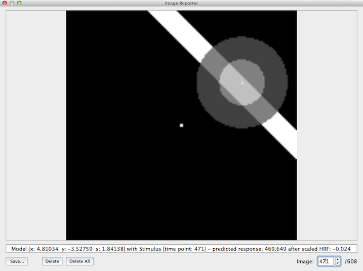
The predicted response at the time point of a stimulus frame is calculated by integrating the weight values in the Gaussian model that overlap with the stimulus. The model has the highest weight value at its center (indicated by a white point within the model) and the weights decrease when moving away from the center as described by the 2D Gaussian function (see topic Introduction). The model-stimulus image shown by the program (example shown above) does not directly indicate the gradual fall off of the Gaussian weights with increasing distance from the center. The fall off is, however, indicated to some extent by showing two disks; the brighter inner disk corresponds to pixels with a distance from the model's center equal or smaller than the standard deviation (1.84 deg in the example); the darker outer disk corresponds to pixels that fall outside 1 standard deviation but inside 2 standard deviations. The area of the model that overlaps with the stimulus is indicated in the example image above by the lighter shaded region where the bar overlaps with the receptive field. In the shown example frame, the sum of all "stimulated" weights leads to a large value of ca. 470 (arbitrary units). At other time points, different values (higher or lower ones) will be produced depending on the model-stimulus overlap. If the stimulus is far away from a considered model (or if no stimulus is shown e.g. in a rest period), a value of 0 would result from the convolution (sampling) process. Note that eac pRF models at different locations and/or with different receptive field sizes will usually produce different response values. In case that enough stimuli with variable position, orientation and sizes are included in the experiment, each model will, thus, produce a unique response time course. In order to compare these model time courses with meausred fMRI data, they need to be convolved with a standard (or individual) hemodynamic impulse response function (HRF). In the example screenshot above, the text line at the bottom of the Image Reporter shows a value after HRF application of only -0.024 despite a high response value for that time point (ca. 470); the reason for this difference is, of course, the effect of the convolution of the produced response time course with the hemodynamic response function, i.e. the response value at a specific frame will have its effect on the predicted BOLD response only several seconds later, i.e. a small value now indicates that there was no stimulus within the receptive field several seconds earlier. The created HRF-convolved time courses (one for each pRF model) will be used as input for the pRF model fitting procedure.
After creating or loading the binary stimulus (.stm) file, the predicted model time courses will be calculated after clicking the Create TCs button. The input spin boxes in the lower section of the dialog is used to specify how many different models should be created. The default entries in the No. of X positions, No. of Y positions and No. of rf sizes spin boxes will generate 30 x 30 x 30 = 27,000 different pRF models and, thus, results in 27,000 predicted model time courses Note that an odd number of x (y) positions need to be entered (e.g. 31) in case that the center point (x=0 degrees, y=0 degrees) should be included in the pRF models. Tests have shown that the default values create enough model time courses to obtain stable pRF estimations for standard fMRI resolution data (i.e. with voxel sizes of 23 - 33 mm3); it seems that good results can already be obtained with smaller values for the x, y, and size parameters, e.g. using values in the range 10 - 20. If desired, the values can also be increased, which is especially useful when using high-resolution data with a resolution of about 1mm x 1mm x 1mm or better. Note that creating all pRF model time courses is a time consuming process involving sampling of each stimulus frame for all 27,000 modes, and it may take an hour or more on standard computer hardware to generate all pRF model time courses (the implementation in BrainVoyager is multi-threaded exploiting multiple processor cores if available). To reduce calculation time, it is also advised to use stimulus frames with a resolution of 100 - 200 pixels (stimulus images with 1 50 x 150 pixels are used in the example described here). [As an alternative, the program could sample only each n'th pixel during stimulus sampling - this is considered for a later release].
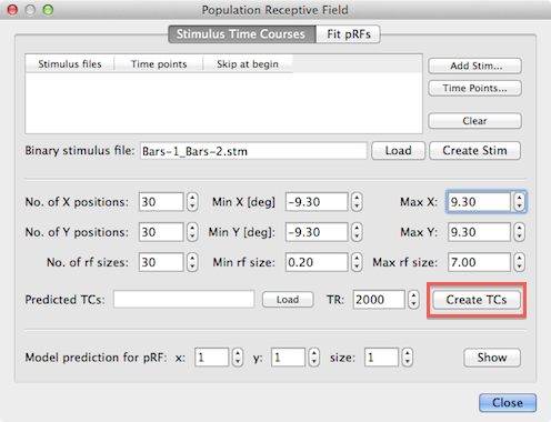
The specified number of x and y positions will be used to create models at equally spaced grid points in the stimulus frames and at each of those grid points the specified number of receptive field sizes will be linearly distributed between the minimum and maximum value provided in the Min rf size and Max rf size spin boxes. In addition to specifying the number of grid points, the mapping from stimulus pixels to degees of visual angle needs to be defined. The value entered in the Min X spin box maps the distance from the center to the left border of a stimulus image to the (absolute) number of degees of visual angle as specified in the Min X spin box while the value in the Max X spin box maps the degrees of visual angle from the center to the right border of the stimulus image as seen by the subject. The same logic applies for the Min Y and Max Y values mapping the distance from the image center to the top and bottom, respectively to degrees of visual angle. Note that the absolute values for the minimum and maximum entries are usually the same. The default values of the minimum and maximum x and y values are 10.0 degrees but they need to be adjusted to the actual values as perceived by the subject in the actual experiment in the scanner. In the example data used here, the values were changed to 9.3 degrees (see snapshot above). The distance of sampled grid points in x (and y) direction can be calculated as d = range/(n - 1) = (max - min)/(n - 1) which results in d = 18.6/29 = 0.64 degrees of visual angle for the example values. The default range of receptive field sizes is from 0.2 to 7.0 degrees of visual angle which results in a step size of 6.8/29 = 0.23. With the number of grid values and the mapping to visual angles the stimulus sampling process for each stimulus frame can be performed but for the final HRF convolution step, the value of the TR (volume time-to-repeat) needs to be entered in the TR spin box. Note that the value is automatically extracted from the header of a selected VTC/MTC files when using the Time Points button as described earlier; if you are unsure about the correct TR value, you may use the Time Points button to select one of the included functional time course files (that all need to have the same TR value) before clicking the Create TCs button.
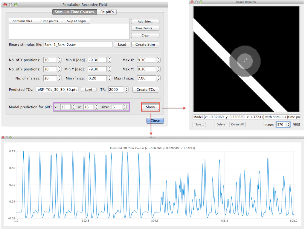
When all pRF model time courses have been created the program saves the created time course in a .ptc (predicted time courses) file for later use. It will generate a name for the file that is based on the file name of the stimulus (.stm) file and it reflects the number of grid positions, receptive field sizes and parameter ranges in degrees of visual angle. If the data has been saved, the given file name appears in the Predicted TCs text field (see snapshot above). It is possible to visualize predicted time courses for specific model pRFs using the Show button in the lower part of the dialog (see snapshot above). The x, y and size spin boxes on the right side of the Model predictor for pRF label can be used to select a specific pRF model. The x, y spin boxes select a position on the internally formed regular grid; in the example, the model with the 15th x position and 16th y position has been selected corresponding to a grid point that is closest to the center on the left side of the x axis and just beyond (i.e. below) the center on the y axis. The corresponding visual angle values are -0.32 and +0.32 as can be seen in the title of the generated time course plot and in the text line in Image Reporter (see snapshot above). After clicking the Show button, the predicted fMRI time course for the selected model is shown in a plot window and the position and size of the receptive field is shown in the Image Reporter dialog. In order to show the overlap of the selected pRF model with any desired stimulus frame, the Image spin box in Image Reporter can be used but only after closing the Population Receptive Field dialog. In the model time course shown above, the first half has a more regular predicted time course than the second half. The reason for this is that in the example data, two runs with bar stimuli were used where the bars were positioned ("moved") over successive spatial positions for a specific orientation sweep in the first run but "jumped" randomly to positions within a sweep in the second run.
As soon as the predicted time courses are generated, the actual population receptive field estimation procedure can be performed in volume space or in cortical surface space.
Notes
It is possible to average VTCs / MTCs of a multi-run pRF mapping of the same scanning session in case that the runs use the same stimulus sequence; it is also possible to average constant sub-sequences within the same run but this currently requires to use the "VTC split" tool to create multiple pseudo-runs. Averaging reduces noise (resulting in higher explained variance values) as well as calculation time since less time points will be used to estimate pRF models.
Copyright © 2023 Rainer Goebel. All rights reserved.