BrainVoyager v23.0
Overlaying Surface Maps on Cortex Meshes
The statistical analysis of functional data is not only possible in volume space but can also be performed on cortical surface meshes providing a more direct view of cortical activation along the gyri and sulci of the brain. Cortical functional analysis is especially important when analyzing topographically organized data such as retinotopic visual field maps or tonotopic auditory maps. The topographical layout of such data can be made even more revealing when inflating and flattening folded cortical surface meshes. The analysis of functional data on cortex meshes is also useful for statistical group analyses since the explicitly represented macro-anatomical folding pattern can be aligned efficiently across subjects using a technique called cortex-based alignment.
There are two major approaches to move from data in volume space to data in cortex space:
- VMP-to-SMP. In the first approach, a folded cortex mesh samples statistical data along the cortex from volume maps loaded on the linked 3D anatomical VMR from which the cortex mesh was derived. This approach is the quckest and easiest way to move to cortex space. An advanced version of this approach is also used for sampling sub-millimeter functional data on cortical depth grids.
- VTC-to-MTC. In the second approach, a folded cortex mesh samples the volume time course (VTC) data along the cortex that is linked to the underlying 3D anatomical VMR creating mesh time course (MTC) data. After sampling, each vertex of a cortex mesh now contains the full time course data of a functional run. The created MTC data can now be (statistically) analyzed in BrainVoyager as any other time course data. A performed single-run GLM, for example, will create statistical surface maps (SMPs) that are overlaid on the cortex mesh. After macro-anatomical alignment, group analyses can also be performed in a cortically aligned space that usually produces better results than conventional group analyses in volume (MNI/Talairach) space.
Since, for conventinoal resolution data, the cortex is modelled as a flat surface (cortical sheet) without depth information, the sampling of voxels onto cortex meshes is an important interface between volume and cortical surface space. BrainVoyager offers several options how to sample functional data when creating surface maps from volume maps directly, or when creating mesh time course data from volume time course data.
From VMPs to SMPs
To directly sample surface maps from volume maps, a cortex (hemisphere) mesh need to be reconstructed from a VMR that is usually normalized to MNI or Talairach space. The volume map(s) need to be calculated and visualized as described in the previous topic, typically by performing single-run GLM statistical analysis. The screenshot below shows on the left side the 3D anatomical VMR document with a overlaid statistical parametric volume map. The right side shows the 3D Viewer window with a loaded cortex mesh of the left hemisphere that has been reconstructed after running a cortex segmentation pipeline.
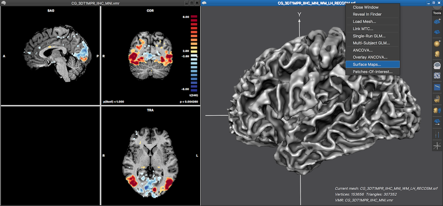
Sampling a surface map from a (overlaid) volume map can be performed in the Surface Maps dialog that can be invoked by using the local context menu in the 3D Viewer window (see screenshot above) or by clicking the Surface Maps item in the Meshes menu. The dialog shows a list of surface maps available for overlay in the Browse tab, which is empty at this stage. In order to create a surface map from the overlaid volume map, the Create SMP button needs to be clicked. This will, however, not start the sampling process immediately but first presents the Depth Integration dialog that allows to specify how the functional data should be sampled.
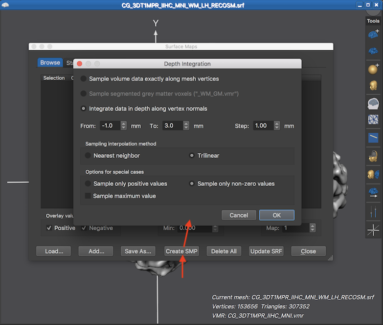
The Depth Integration dialog offers three approaches how the mesh samples the underlying functional data in the associated volume space. When selecting the Sample volume data exactly along mesh vertices option, no depth integration is actually performed, i.e. the vertices will contain the data from the voxels in volume space that are closest to the loation of the mesh vertices. If this option is combined with the Nearest neighbor interpolation option in the Sampling interpolation method field, a single vertex simply copies a (statistical) value from the closest voxel in volume space. This approach might be preferred in cases that one wants to ensure that the original map values are not changed when putting them on a surface mesh. It is, however, generally recommended to select the (default) Trilinear interpolation option since vertices after mesh smoothing do not sample the centers of voxels but sample in-between voxels and trilinear interpolation more appropriately reflects the smoothed geometry of the cortex mesh.
The Sample segmented grey matter voxels option and the Integrate in depth along vertex normals opton also sample from voxels close to the location of mesh vertices but values are integrated along the normal of a vertex, i.e. along the direction that is orthogonal to the surface area around a vertex. Since the mesh surface extends tangentially along the cortex, sampling along the vertex normal, thus, integrates data along the depth of the cortex. Since the cortex has a thickness in the range of 2-5 mm, depth integration is relevant even with a standard resolution of 2 mm voxels. The range of sampling along the normal can be specified for the Integrate in depth along vertex normals option. The entry in the From value box specifies where to start the depth sampling process with respect to the coordinates of a vertex, i.e. the default value of -1.0 starts the depth integration 1 mm "backwards" towards white matter. The default starting value is not set to 0.0 since it is assumed that a "RECOSM" mesh is used as default which typically runs not exactly along the white-grey matter boundary but about 1 voxel (usually corresponding to 1 mm) inside grey matter. In case that a cortex mesh is used that runs exatly along the white-grey matter boundary (e.g. a "WM" mesh), a value of 0.0 can be used in that field. From the specified starting point, sampling along the normal proceeds with a step size in millimeter that is specified in the Step value box. The default value for the To field is set to 3.0, i.e. depth integration proceeds up to 3 mm through grey matter towards CSF. Note that voxels are excluded from depth integration if they do not have a non-zero value in case that the Sample only non-zero values option is turned on (default). Another option to sample the best data along the vertex normal is to select only the encountered maximum value. If this Sample maximum value option is turned on, no depth integration (averaging) takes place since only a single value is selected as with the "sample exactly along mesh vertices approach" but from all values sampled along the normal, only the "best" value is retained, i.e. the one with the highest absolute value.
The Sample segmented grey matter voxels option (added in BrainVoyager 21.0) implements a similar approach than the Integrate in depth along vertex normals option. The difference is that the depth sampling range need not to be specified since it is automatically limited to grey matter voxels. This option thus does not require specifiying the sampling range along the normal and it is particularly useful in light of the fact that the cortex varies in thickness. Note that the option is disabled in the screenshot above since it requires an associated VMR volume with an explicit labelling of grey matter voxels. More specifically, grey matter voxels need to have the intensity value of 100. Since the automatic advanced segmentation pipeline produces a file with explicit grey and white matter labels (with values 100 and 150 respectively), the option is turned on only if the file name of the associated VMR volume ends with the "_WM_GM.vmr" substring as indicated in brackets at the end of the name of this option. If one does not have such a VMR file, one can also use the region growing tool in the 3D Volume Tools dialog to approximately label grey matter voxels, saving the resulting VMR file under a name ending with the "_WM_GM.vmr" substring.
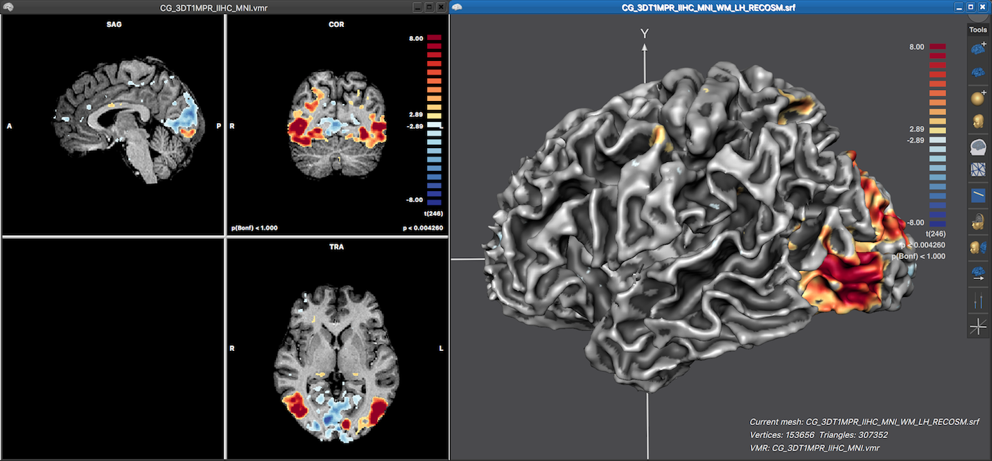
The screenshot below shows the resulting surface map overlaid on the left hemisphere cortex mesh after clickng the OK buton in the Depth Integration dialog using all default settings, i.e. keeping the selected Integrate in depth along vertex normals option and all other sampling options. Note that the the displayed surface map nicely reveal in 3D how the statistical map data extends along the cortex. Also the map colors look similar as in the volume map on the left side since the same functional look-up table (LUT) is used automatically. Since no LUT has been specified explicitly for the volume map, the default color range is used for the volume map and thus also for the surface map. The LUT can be changed for both volume and surface maps in the Confidence range field in the Statistics tab of the Volume Maps and Surface Maps dialog, respectively.
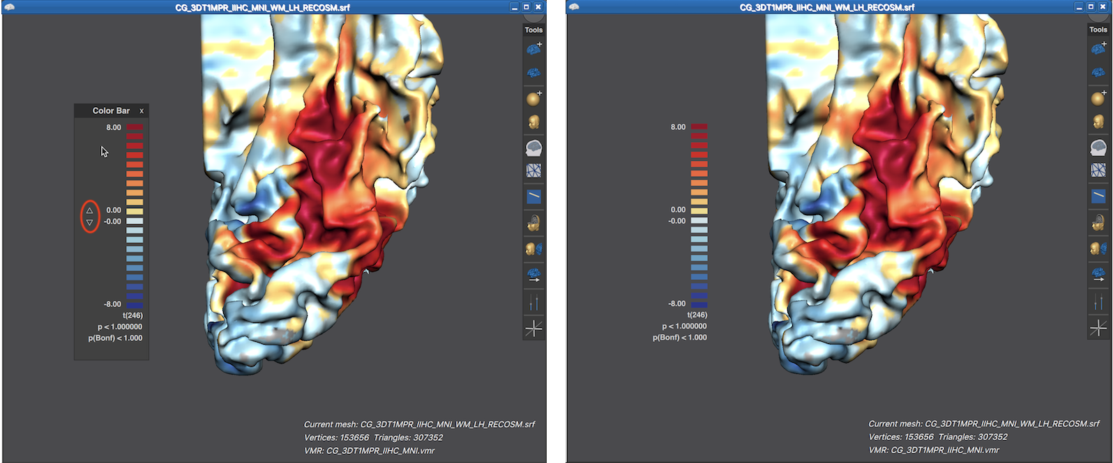
Note that the displayed LUT color bar in the 3D Viewer appears as "baked" in the background. The color bar is, however, the content of a Color Bar panel as can be revealed by moving the mouse pointer over the color bar (see screenshot below).
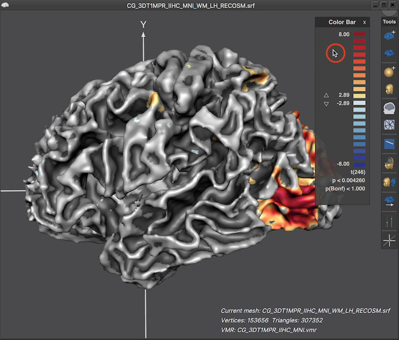
When the title bar and background area of the Color Bar panel is visible, the panel can be moved inside the 3D Viewer like any other panel. Furthermore up and down buttons are revealed that can be used to change the threshold of the overlaid surface map (see screenshot below). When moving the mouse pointer out of the panel, its title bar and background area disappear again, which provides a nicer look for preparing figures. In the screenshot below (left side), the viewpoint has been changed to reveal activity in ventral visual cortex of the cortex mesh. Furthermore, the Color Bar panel has been moved from its default location to the left side and the revealed threshold buttons have been used to set the threshold value to 0.0, which shows the surface map unthresholded, i.e. over the whole mesh. The right side below shows the same situation after moving the mouse pointer out of the Color Bar panel.
Note that the threshold of the surface map as well as man other settings can be controlled from the Surface Maps dialog.
From VTCs to MTCs
When going from volume to cortical surface space using the time course approach, the first preparatory steps are the same as for the surface-from-volume-map sampling approach, i.e. an anatomical VMR document needs to be available and a cortex mesh needs to be loaded into the 3D Viewer that has been reconstructed from the brain in the VMR document window. Instead of loading volume maps, one needs to link a volume time course (VTC) file to the VMR document. In order to initiate the sampling process, the Mesh Time Course dialog can be used, which can be launched by selecting the Mesh Time Course item in the Meshes menu. The dialog opens with its first Link MTC / SSM tab selected. Switching to the Create MTC from VTC tab reveals the same sampling options that have been described above. After modifying or keeping the sampling options, the sampling process can be started by clicking the Create MTC button. The resulting MTC file can then be linked to the current mesh by using the Link MTC item in the title bar's context menu of the 3D Viewer or by using the Browse button on the right side of the MTC file item in the Mesh time course file field in the Link MTC / SSM tab of the Mesh Time Course dialog. For more details, see topic From Volume to Mesh Time Courses.
The created MTC file can now be used to perform a single-run GLM analysis, which will generate a statistical map for the omnibus GLM test (contrast with all main condition predictors set to 1) that will be shown as a surface map on the cortex hemisphere mesh.
Copyright © 2023 Rainer Goebel. All rights reserved.