BrainVoyager v23.0
Reconstructing Edited Brain Volumes
While cortex meshes are reconstructed automatically when running the standard and advanced segmentation pipelines, it is often necessary to reconstruct segmentations that have been manually edited using manual segmentation tools. This can be done using the 3D icon in the Zoom View toolbar for multiple segments. Here the most basic approach is described using one segmentation labelled with the default "blue" segmentation color (value 240). The segmentation typically represents one cortical hemisphere after manual editing but the procedure is general and can be used for any segmented volume. After preparing the boundary of the segmented structure (see below), the mesh reconstruction process is performed from the 3D Viewer either by using the Reconstruct Mesh From Prepared Volume icon or via the Create Mesh dialog.
In case the volume is not an (manually edited) VMR resulting from a segmentation pipeline, a desired volume need to be first marked as a segmentation using the tools in the Segmentation tab of the 3D Volume Tools dialog. This usually involves application of region growing and the range tool to remove voxels with intensity values of no interest. Region growing is prepared by clicking inside the to-be-segmented volume to specify a seed voxel with high enough signal intensity for a region growing operation. Region growing spreads from the voxel to those voxels that are in the intensity range specified by the the Min entry and the Max entry in the Value range. Useful values for white matter are typically in the range of 120-180 but the values depend on the specific anatomical data and the preprocessing performed. Running the intensity inhomogeneity correction procedure is highly recommended if not already performed prior to standard cortex sgementation pipelines. Note that the intensity of the seed voxel must fall within the specified range, otherwise the segmentation will not spread to neighboring voxels. The region growing process is started by clicking the Grow Region button. If the result is not optimal, i.e. does not include the voxels of the desired volume, the minimum and maximum range values can be adjusted before repeating the process. When manually editing an already segmented brain hemisphere volume, region growing is not necessary.
In case one uses other labeling colors than the "blue" segmentation color, the range tool can be used to map those other colors either as belonging to the segment or to remove them by mapping them to a value of 0 intensity. Note that the "intensitiy values" beyond 225 (226-255) are not used to represent actual intensity values but are used as special values for segmentation (and other) purposes.
Starting with Non-Segmented Volumes
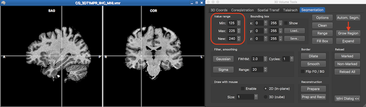
The screenshot above shows a non-segmented volume that has been normalized to MNI space after only applying the standard intensity inhomogeneity correction tool including the default brain extraction step. In this case a simple segmentation can be produced using the region growing tool. The target here is to roughly segment a whole-brain white matter volume. The cross has been set at a voxel inside white matter (see above) serving as the seed voxel for the region gowing process. In order to detect intensity values of the target structure, it is useful to hover the mouse over the voxels that are located inside and outside the target structure, and especially at the transition between the target and nighboring structures (e.g. grey matter). When hovering the mouse over voxels, the intensity value at the voxel under the mouse pointer is printed in the status bar and the inspected values in neighboring structures can serve as hints for the range values entered in the Value range field. In this example the value 125 has been entered in the Min box and value 225 for the Max box. The label color that will be used during region growing is set in the New box and should have the defautl segmentation value of 240. The screenshot below shows the resulting labelling after clicking the Grow Region button.
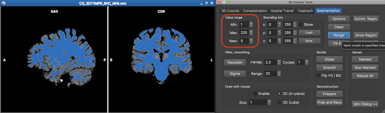
In case the results of region growing are not as expected, it is advised to adjust the minimum and maximum range values in the Value range field and start again after clicking the Reload All button which reloads the original (unsegmented) volume from disk. If the region growing segmentation is acceptable, one needs to remove unwanted tissue before the volume can be reconstructed as a mesh. On the right side in the screenshot above this is already prepared by using again the Value range field but this time combined with the range tool. The range tool maps all voxels in the volume (eventually restricted by the values in the Bounding box field) with intensities from the minimum to maximum value (inclusive) to the intensity value in the New number box. Since the segmentation value of 240 is beyond the used intensity values (0 - 225), the range is set to a minimum value of 1 (or 0), a maximum value of 225 and a resulting value of 0. When clickiing now the Range button, all voxels will be set to 0 except the blue marked voxels as shown in the screenshot below.
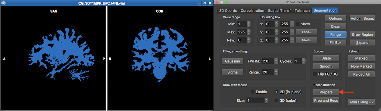
The obtained segmentation with only blue labeled voxels could be further enhanced (e.g. by filling holes, border smoothing and morphological operations). At any moment one can convert the current segmentation state into a mesh representation. This requires clciking the Prepare button, which executes a process that labels the voxels at the outside fringe of the segmented structure with a yellow color (value 235). Note that when editing the volume, this preparation step need to be always performed in order to obtain a correct boundary representation for subsequent mesh reconstruction.
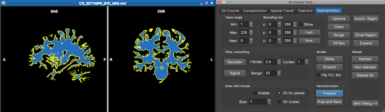
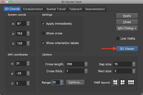
The prepared segmented volume (with only blue colors and a yellow outline) can be reconstructed using the 3D Viewer window, which can be launched by clicking the 3D Viewer button in the 3D Coords tab of the 3D Volume Tools dialog (see snapshot below).
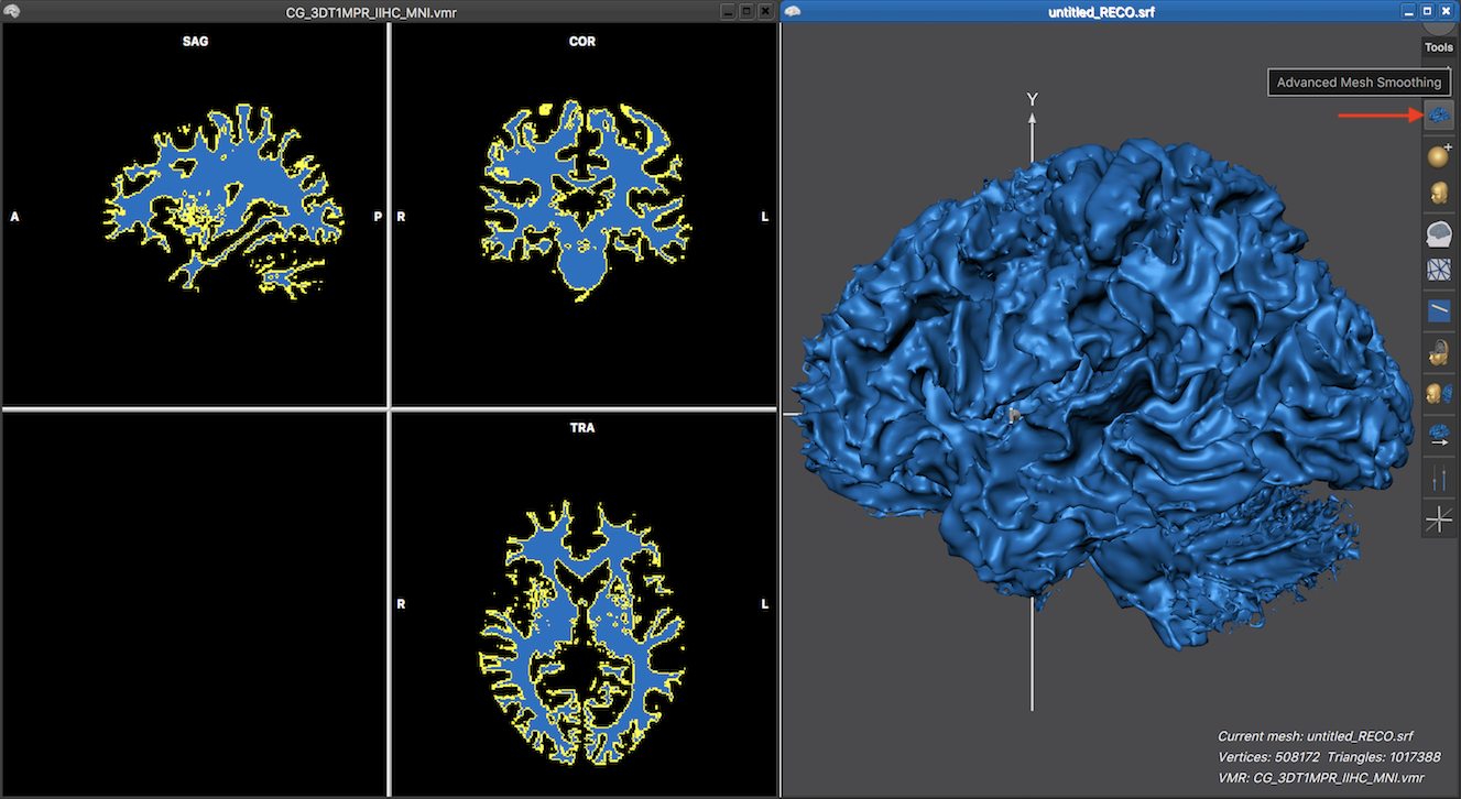
The mesh reconstruction can then be performed simply by clicking the Reconstruct Mesh From Prepared Volume icon in the 3D Viewer (see snapshot below). In a couple of seconds the mesh will appear in the 3D Viewer. The screenshot below shows the reconstructed mesh on the right side and the used segmented structure in the associated VMR document window on the left side. Note that the mesh can also be reconstructed using the Create Mesh dialog which can be invoked from an active 3D Viewer window by clicking the Create Mesh item in the Meshes menu.

As one can see above, the reconstructed mesh looks very blocky since the reconstructed boundary consists of a triangulation of voxel faces that continue either in a straight direction from voxel to voxel or meet at 90 degree angles resulting in the blocky appearance. In order to obtain a more smooth approximation of the reconstructed boundary, a non-shrinking smoothing step can be launched by clicking the Advanced Mesh Smoothing icon which is located directly under the Reconstruct Mesh From Prepared Volume icon (see snapshot below).
The resulting mesh reconstruction now shows a smoothley curved surface. Note that the applied advanced smoothing limits smoothing to high-frequency geometry changes in order to keep the low-frequency information (e.g. the macro-anatomical folding pattern of gyri and sulci) intact. This is in contrast to standard smoothing operations (as is available in the Mesh Morphing dialog) that also removes low-frequency information; standard smoothing is, however, important as part of mesh inflation, flattening and mesh-to-sphere morphing.
Starting with (Edited) Segmented Volumes
The section above described basic segmentation tools and how segmented volumes are prepared for surface reconstruction. It then showed how a mesh surface is reconstructed from the prepared volume. In the context of creating topologically correct left and right hemisphere meshes, one typically starts with already prepared segmented volumes of the left and right white matter and only tries to remove remaining issues in the segmentation that could not be handled by one of the automatic segmentation procedures. In this case the following steps are typically applied:
- Edit blue/yelllow white matter segmentation of (left or right) cortex hemisphere in the volume
- Prepare the volume for surface reconstruction using the Prepare button as described above
- Reconstruct and smooth the mesh in the 3D Viewer as described above
- Optional: Project the mesh in the volume and inspect the original intensity data loaded as a secondary/tertiary volume to the VMR document containing the segmented volume
- Inspect the mesh for remaining topologically errors
- If no more issues are detected, editing is done and the reconstructed cortex hemisphere mesh can be used for further processing, e.g. for cortex inflation or cortex-based alignment. In case there are additional issues, go back to step 1
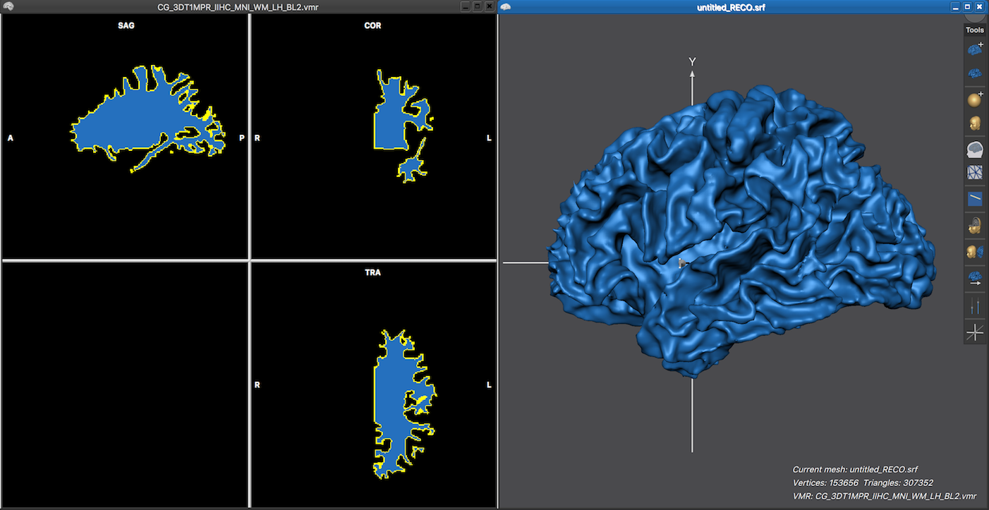
The left side in the screenshot below shows the white matter segmentation result of the left hemisphere of the brain used in the example above after running the standard segmentation pipeline. Since the bridge removal tool was included in the segmentation pipeline, the VMR file name contains the "_BL2.vmr" file extension. The right side in the screenshot below shows the reconstructed and smoothed mesh surface, which appears without topological errors.
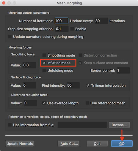
A recommended approach to detect topological issues is to partially inflate the mesh using the Mesh Morphing dialog (see below), which can be invoked by clicking the Mesh Morphing item in the Meshes menu. In order to tell the mesh morphing routine to perform mesh inflation, check the Inflation mode selection box (see screenshot below). To start the inflation process, click the GO button. Note that you may set a low value (e.g. 100) in the Number of iterations text field before starting the morph process but inflation may also be interrupted under visual inspection by pressing the ESCAPE key or by cancelling the appearing morphing dialog.
The screenshot below shows the partially inflated mes in the 3D Viewer on the right side, which now reveals a few minor issues that one may want to correct. Note that he link between the mesh and the VMR document allows to locate the region in the VMR document by simply clicking close to the issue on the mesh. This is indicated by the red arrows, which show the location of a performed mouse click and the resulting automatic resliced volume on the left side with the white cross pointing at the respective position.
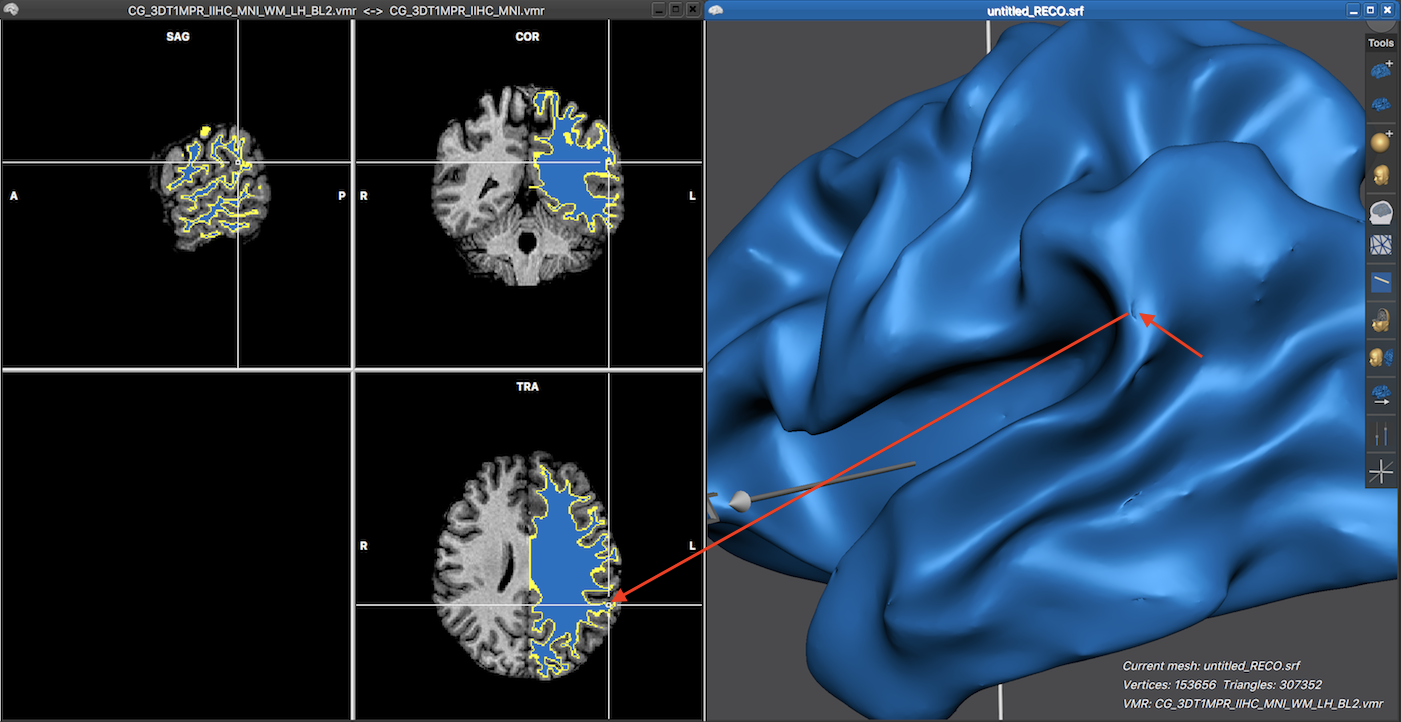
Note that the left side not only shows the prepared segmentation volume but also the original normalized VMR document, which has been loaded as a secondary document. For more information on how to correct topographical issues, check topics Verification of Segmentation Results and Manual Segmentation Tools.
Copyright © 2023 Rainer Goebel. All rights reserved.