BrainVoyager v23.0
Boundary-Based Registration
Since BrainVoyager 20.2 boundary-based registration (BBR) is available as a powerful method to coregister anatomical data with functional (and other) data sets from the same subject. BBR uses a cortex mesh reconstructed along the white-grey matter (WM/GM) boundary of the anatomical data to drive the alignment by projecting the mesh in the functional (or other) data set and by spatially transforming the mesh until its vertices align with the maximal intensity gradient across white and grey matter in the functional data set (Greve & Fischl, 2009). This approach requires that the anatomical dat set is of sufficient quality and spatial resolution to derive a cortex mesh from segmented white-grey matter boundary. Since the derived cortical surface drives the alignment, the target (functional) data sets need not be of high quality (as compared to the anatomical data set) but they must differentiate grey and white matter to form tissue intensity gradients across the WM/GM boundary. BBR leads usually to optimal alignment results that are of better quality than those achieved with other approaches using image intensity or image gradients to drive alignment. Furthermore, BBR is a very robust alignment mechanism since it only operates at locations of the projected cortical surface ignoring voxels that are not close to the mesh boundary. BBR is also robust with respect to spatial intensity inhomogeneities in the target (e.g. functional) data sets since it calculates tissue intensity gradients locally. Its high robustness also allows to align partial (functional, diffusion-weighted) volumes to anatomical data sets, which is useful e.g. for the analysis of high-resolution data that often covers only a small slab of the brain.
Note that BBR aligns the cortical surface (representing the WM/GM boundary of the source anatomy) to the target (e.g. functional) data set. The inverse is, however, often desired i.e. to align the functional data to the anatomy. Since BBR implements a rigid alignment (eventually with scales, see below), the produced spatial transformation matrix can be used both forward (from the anatomy to the functional data) as well as backward (from the functional data to the anatomical data). Furthermore, a special spatial transfomration file is produced that can be used for the fine-tuning alignment step of the standard FMR-VMR coregistration.
Because of the excellent alignment results, BBR is now provided as the recommended option for many standard alignment tasks:
- Fine-tuning adjustment (FA) when coregistering functional (or diffusion-weighted) data of runs with an anatomical data set from the same scanning session. BBR can now be used instead of the other available approaches that are based on gradient or intensity-driven coregisttration. BBR is also available in the FMR-VMR Coregistration sub-workflow in the data analysis manager.
- Multi-run coregistration. When using BBR, it is recommended to align each individual run of a scanning session to the native VMR data set and to use the produced FA matrix for the respective run. It is thus not necessary (and not recommended for BBR) to use across-run motion correction since the FA transformation files produced by BBR for each run will handle the run-to-run displacements caused by head motion.
- Native-space VMR alignment with FMR-VTC Space. In case functional data is analyzed in FMR-VTC space (e.g. when analyzing high-resolution data), the functional data is not aligned to the native space VMR. Instead, the native-space VMR is transformed into the original FMR-VTC space. Alignment of multiple runs needs also special treatment that can be based on BBR.
- Creation of mesh time course (MTC) data from volume time course (VTC) data can now be optimised using BBR.
The topics referenced in the application list above provide specific instructions how to use BBR. A more detailed general description of BBR is provided below.
Background
BBR assesses the state of alignment for a given set of spatial transformation parameters (3 translations and 3 rotations as default) by calculating a cost function using the locations of the vertices of the white/grey matter cortex mesh in the target volume (usually a volume of T2 weighted functional data). As long as the optimization procedure finds transformation parameters that decrease the cost function, the optimization procedure continues, otherwise it stops reporting the obtained cost function before and after alignment in the Log tab.
The cost function integrates local calculations around vertices projected in the target (e.g. functional) volume (see figures above and below). A single vertex contributes to the cost function by calculating a gradient value that is obtained by subtracting sampled intensity values on both sides of the vertex when moving along its normal (a normal vector is oriented in an orthogonal direction with respect to the orientation of a local surface patch around the vertex). In the figure below, the sampled grey matter intensity value for vertex v is denoted g and the sampled white matter intensity value is denoted w. The step size into grey and white matter is usually set to 1.5mm but it can be changed in the Boundary-Based Registration dialog. The gradient is then simply calculated as gradv = gv - wv. where the subscript v refers to the specific vertex considered. The figure below shows the relevant information for a single vertex while the figure above shows the
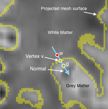
If we assume good registration, the vertex will be located at the white/grey matter boundary and the normal will point "outside" into grey matter and its inverse direction will point "inside" into white matter (see figure above). The difference between the two sampled values will be large and they will have the same sign across vertices (e.g. always positive) in case of good alignment; if the mesh is not (yet) aligned with the target volume, the sign of the gradient will be inconsistent across vertrices (positive and negative values) or the gradient will have values around zero in homogeneous tissue; both factors will lead to a much smaller average value as compared to the case of good alignment. More specifically the local contrast function C for vertex v is caluclated as follows:
Cv = 100 * (gv - wv) / ((gv + wv)/2)
Note that the gradient is normalized by dividing the difference of the sampled grey and white matter value by the average of the two values. Since the resulting value is also multiplied by 100, the resulting value of a vertex is expressed as a percent contrast value. These values could be averaged to obtain a mean percent value as a measure of goodness of registration but the resulting average would still depend on the tissue contrast of the target volume. In order to obtain a robust global cost value that integrates local cost largely independent of local tissue contrast, the percent contrast values are "squeezed" between value 0 and value 2 by calculating the local cost function J for vertex v as:
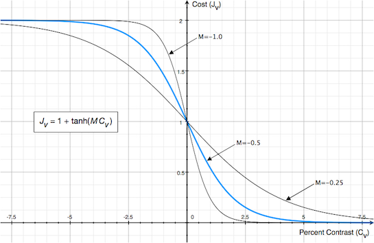
Jv = 1 + tanh(M Cv)
A percent contrast value of 0 results in a local cost value of 1, a large percent contrast value in the right direction leads to a cost close to 0 and a large percent contrast value in the wrong direction leads to a cost close to 2 (see graph below). The absolute value of parameter M (default 0.5) determines how fast values go down to 0 or up to 2 with increasing (decreasing) percent contrast values. The sign of M is important since it needs to be consistent with the tissue weighting of the target volume, i.e. grey matter values are larger than white matter values in T2 weighted images while the reverse holds in T1 weighted images. The value of the overall cost function J is simply the average of all vertex cost values.
The cost value before starting alignment and after BBR completes are written in the Log tab together with the spatial transformation parameters leading to optimal alignment. Furthermore, these parameter values are also saved to disk as standard TRF files in two versions; one version ending with the string "_FA.trf" is prepared as the fine-tuning transformation matrix that can be used, e.g. in subsequent VTC creation. The second TRF file ending with the string "_3D3D.trf" can be used for other 3D-3D transformation; if applied normally (forward) this can be, for example, used to transform the native-space anatomical VMR into the space of the target (e.g. functional) volume; the same matrix can also be used to transform the derived cortex mesh into the space of the target volume. The transformation matrix can also be applied backwards to align the target volume into the space of the source volume or cortex mesh.
Note that the value of the cost function will be typically in the range of 1.0 - 1.2 in case that the cortex mesh is not well aligned with the target VMR. If projected in standard functional data sets (e.g. 2 mm EPI data), typical values after BBR are in the range of 0.3 - 0.5. In case that the cortex mesh is projected in a T1 weighted anatomical data set (from the same or different session) values below 0.1 are usually observed. A value of the cost function around 1.0 before and after BBR indicates that alignment did not work typically because some prerequisites are not met; it could be, for example, that the mesh is to far off from the WM/GM boundary of the target volume, which can be checked by projecting the mesh in the target VMR; it could also be that the tissue intensity gradient is calculated in the wrong direction, which can be resolved easily by flipping the respective grey matter vs white matter option in the BBR dialog (see below).
General Application of BBR
The application of BBR requires some preparatory steps that are not needed when using image intensity based alignment techniques, most importantly, a white/grey matter segmentation of the anatomical data set needs to be performed in order to derive a surface that models the white-grey matter boundary. In order to make this task as simple as possible an automatic cortex segmentation tool is provided that uses a (native-space) VMR as input and produces a whole-cortex mesh as output suitable for BBR application. Details about this tool are described in the topic Automatic Cortex Segmentation for BBR. The resulting cortex mesh (example shown in the snapshot below) will not be a (topologically) perfect WM/GM surface, i.e. it will contain subcortical structures and the cerrebellum and it will likely have several topological errors. As long as the mesh reconstructs the white/grey matter boundary in most places, these issues will not have a negative impact on the quality of the subsequently performed BBR alignment due to its high robustness and tolerance to segmentation errors.
Besides a reconstructed mesh, the target (e.g. functional) data must be available in a VMR file with the same spatial resolution as the cortex mesh. To run BBR, the target volume needs to be loaded first serving as the underlying (hosting) VMR for the cortical surface. Specific BBR application routines (FMR-VMR alginment, MTC creation) ensure that an adequate VMR file containing the (functional) data is created. In case that VTC (or VDW) data in some sapce is available, an appropriate VMR can also be created directly using the Show VTC Vol button in the Spatial Transf tab of the 3D Volume Tools dialog. This function ensures that the VTC/VDW data is interpolated to the same resolution as the hosting VMR. The generated VMR is stored as a secondary volume (attached to the primary VMR) and can be saved to disk using the Save Secondary VMR item in the File menu.
With the BBR target volume selected as the active document, the created white matter cortex mesh of the subject's brain is loaded and will be visible in the standard surface (OpenGL) window. In order to check that the mesh is indeed suitable to be used for BBR, it is recommended to project the mesh in the underlying volume. BBR wil usually work if the visualized mesh contours are in proximity to the white-grey matter boundary of the (functional) data stored in the hosting VMR. When using some of the specific applications mentioned above, the necessary proximity will be ensured by appropriate preparatory steps (such as initial header-based alignment).
With the desired target VMR and loaded cortex mesh, BBR can be performed using the Boundaery-Based Registration dialog that can be invoked by clicking the Boundary-Based Registration item in the Meshes menu. The selections made as default in this dialog are well prepared and usually need not to be changed, i.e. the process can be started directly using the GO button. If not using standard functional data sets, the only important option is related to the white/grey matter intensity weighting (see below).
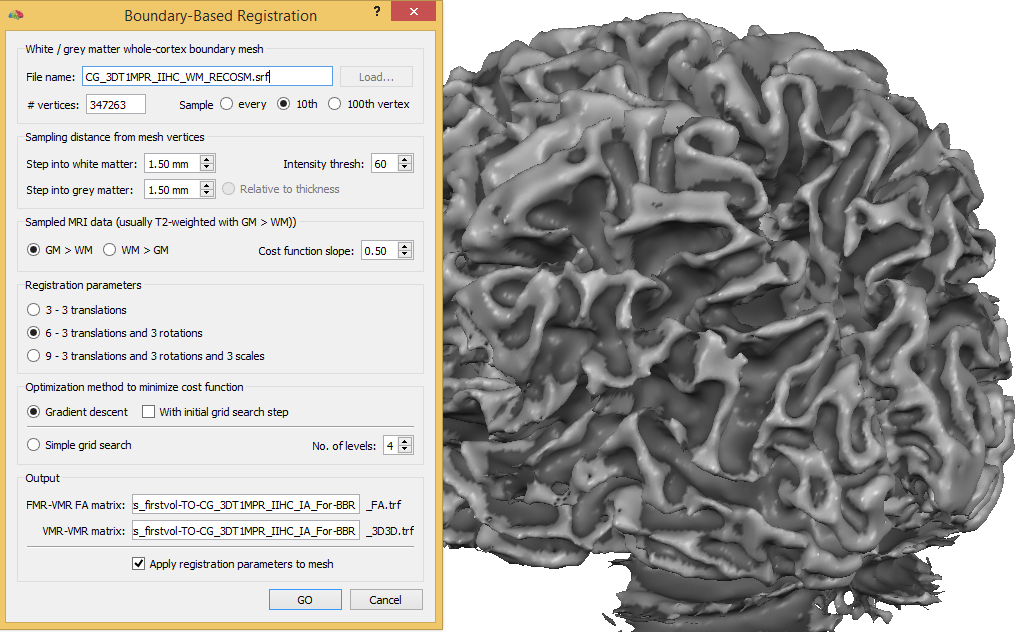
At the top of the dialog the name of the currently loaded mesh is shown in the White / grey matter whole-cortex boundary mesh field. The number of verticers of the mesh is displayed in the # vertices field; this information is useful to decide whether all vertices should be used for driving the alignment or whether a subset is sufficient. Since reconstructed whole-cortex meshes usually contain at least 300,000 vertices, the default option Sample every 10th vertex is recommended since it has been shown that results do not differ substantially than using the Sample every vertex option. In case high-resolution meshes are created that are not simplified (with e.g. more than a million vertices), the option Sample every 100th vertex should be used to save processing time. The Sampling distance from mesh vertices field can be used to adjust the distance from a vertex along its normal to sample into white matter ("inside" direction) and grey matter ("outside" direction) using the Step into white matter field and Step into grey matter fields, respectively. The default values of 1.5 mm have been tested extensively and work fine in most cases (in a future version the inside grey matter step wil be also adaptive based on cortical thickness measurement).
The Sample MRI data field is important since it can be used to adjust to the tissue weighting. The default option GM > WM is intended for the most usual case where the underlying VMR contains a functional data volume that have higher intensity values for grey matter than for white matter. BBR can however also be used for other MR pulse sequence that may have higher values for white matter than for grey matter. If one wants, for example use BBR to align to a T1 weighted anatomical data set of the same subject, the WM > GM option needs to be selected in order to produce correct results. The Sample MRI data field also contains the Cost function slope field that can be used to adjust the function that converts the calculated tissue contrast of a vertex into a cost function value (for more details, see Background section above).
The Registration parameters field can be used to determine which spatial transformation parameters of the mesh are allowed to be changed in order to optimize alignment. As default, a rigid alignment with 3 translations and 3 rotations is chosen (option 6 - 3 translations and 3 rotations) since the two data sets are assumed to come from the same brain. Due to small distortions, it might be beneficial to add scaling parameters (9 parameter option 9 - 3 translations and 3 rotations and 3 scales). The 3 parameter option 3 - 3 translations may be useful when one wants restrict alignment solely to translations.
The Optimization method to minimize cost function field can be used to select either a gradient-descent optimization approach (Powell method, ref) or a grid search approach. The Gradient descent optimization method is selected as default since there is usually only one global minimum of the cost function if the procedure is started with a mesh sufficiently close to the target white/grey matter boundary. In case that the mesh deviates more than 4-5 millimeter/degrees from the target white/grey matter boundary, it is advised to turn on the With initial grid search step option. The gradient descent technique is advised since it finds the minimum reliably and since it requires much less time than when using the Simple grid search option. In case that the overall cost function value does not go substantially below 1.0, it is advised to check whether the tissue weighting option in the Sample MRI data field is set correctly.
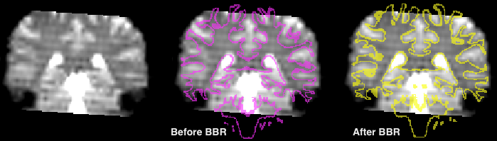
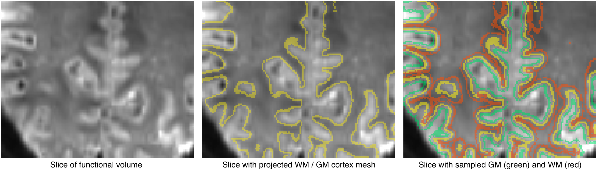
The Output field contains text fields with the suggested names of the spatial transformation (TRF) files that will be produced as the result of BBR. The FMR-VMR FA matrix TRF file is a special version of the calculated spatial transformation that can be used for fine-tuning alignment in the standard FMR-VMR coregistration procedure. The VMR-VMR matrix TRF file can be used to transform the source VMR file or the source mesh into the target (e.g. functional) VMR space. This matrix can also be used backwards to bring the target VMR (containing e.g. a representation of a functional volume) into the source space. This is also important when performing multi-run alignment for high-resolution (sub-millimeter) data sets. The calculated spatial transformation is applied to the source cortex mesh in case the option Apply registration parameters to mesh is turned on (default); furthermore the mesh is projected in the target VMR before and after BBR (represented as two VOIs) allowing to visually assess the achieved coregistration quality. The snapshot above shows a typical BBR result for a coronal slice of the target VMR of a functional volume; on the left side the coronal slice is shown without the projected mesh contour, the middle panel shows the projected mesh before BBR (VOI with pink color) and the right panel shows the projected mesh after BBR (VOI with yellow color) has been performed. It is obvious that the mesh contour much more precisely follows the transition from white (darker intensiy colors) to grey (brighter intensity colors) tissue much more precise after BBR (right panel) than before BBR (middle panel).

Besides the spatial transformation (TRF) files, the achieved alignment quality and transformation parametrs are also written in the Log panel. The snapshot above shows three text lines produced by the BBR procedure. The first line informs about the cortex mesh and the target volume used for alignment. The second row shows the cost function before running BBR, i.e. usually after header-based alignment and the third line shows the cost function after BBR as well as the respective spatial transformation parameters used to achieve the alignment. The example output abvoe shows that the cost function was reduced from a value of 0.6 before BBR to a value of 0.38 after BBR, which reflects a substantial improvement of alignment of the mesh with the white/grey matter tissue border in the target functional data volume.
References
Greve D, Fischl B (2009). Accurate and robust brain image alignment using boundary-based registration. Neuroimage, 48, 63-72.
Copyright © 2023 Rainer Goebel. All rights reserved.