BrainVoyager v23.0
Support Vector Machines (SVMs)
One of the most popular MVPA tools are based on support vector machine (SVM) classifiers. SVMs have become the method of choice to solve difficult classification problems in a wide range of application domains. What makes these classifiers so popular? Their "fame" mainly rests on two key properties: 1) SVMs find solutions of classification problems that have "generalization in mind", and 2) they are able to find non-linear solutions efficiently using the "kernel trick".
The first property leads to good generalization performance even in case of high-dimensional data and a small set of training patterns. This is very relevant for fMRI applications since we typically have many features (voxels), but only a relatively small set of trials per class. While this SVM property is useful to reduce the "curse of dimensionality" problem (see topic Basic Concepts) by reducing the risk of over-fitting the training data, it is still important to reduce the number of voxels as much as possible. In machine learning, this feature reduction step is referred to as feature selection. One way of feature selection consists in restricting the number of voxels to the ones in anatomically or functionally defined regions-of-interest (ROIs).
The second property is important to solve difficult problems, which are not linearly separable. A binary (i.e. two-class) classification problem is called linearly separable, if a "hyper-plane" can be positioned in such a way, that all exemplars of one class fall on one side and all exemplars of the other class fall on the other side. In case of two feature dimensions (e.g. two voxels), the "hyper-plane" corresponds simply to a line, in case of three features, the hyper-plane corresponds to an actual 2D plane. The term "linear" means that the separating entity is "straight", i.e. it may not be curved. In difficult classification problems, optimal solutions may only be found if curved (non-linear) separation entities are allowed. In SVMs non-linear solutions can be efficiently found by using the "kernel trick": The data is mapped into a high-dimensional space in which the problem becomes linearly separable. The "trick" is that this is only "virtually" done by calculating kernel functions. For problems with high-dimensional feature vectors and a relatively small number of training patterns, non-linear kernels are usually not required. This is important for fMRI applications, because only linear classifiers allow to interpret the obtained weight values (one per voxel) in a meaningful way for visualization and feature selection (see below).
Large-Margin Separation - The Hard Margin Case
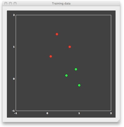
To understand why SVMs lead to good generalization performance, let's consider a simple example consisting of 6 patterns with only two features, allowing to visualize the patterns in 2D space. In the figure above, each point represents one training pattern. The x component of a point corresponds to its value on feature 1 and the y component corresponds to its value on feature 2. In the context of fMRI data, the 6 points would correspond to 6 trial responses with estimated response amplitudes in two voxels. The red points belong to class 1 and the green points belong to class 2. In the fMRI context, the red points correspond to patterns evoked by trials from a different condition ("red condition") than the green points ("green condition"). In machine learning terminology, the assignment to a class is referred to as a "labeling". For binary classification problems, the labels are typically "+1" for the "positive" class (e.g. red points) and "-1" for the "negative" class (e.g. green points). BrainVoyager stores the feature values and their labels in a new "MVP" (multi-voxel patterns) file format. The "example1.mvp" data file producing the figure above contains the following lines:
FileVersion:   1
NrOfExemplars: 6
NrofFeatures:  2
+1   0.7  1.0
+1   0.1  0.7
+1   0.3  1.4
-1   0.9  0.3
-1   0.6  0.1
-1   1.0 -0.2
Following the specification of the number of exemplars (patterns) and the number of features (voxels), each line in the file contains one pattern together with the corresponding class label, which appears in the first column. This format is the same also for real data, but the number of features (voxels) will be usually much higher (see below).
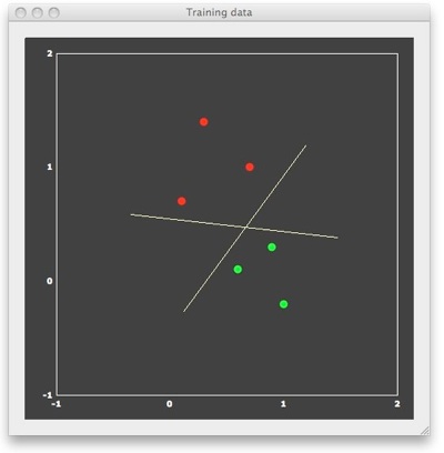
We can now "train" a SVM classifier by providing it with the 6 patterns and associated labels as input. The result of this supervised learning will be a decision boundary (a straight line in the linear case) separating the two classes. When looking at the figure above, it is obvious that there are many lines, which would correctly separate the two classes. Many classifiers (e.g. most neural networks) would present separating lines as shown in the figure above, but SVMs strive for an "optimal" separating line, which should be as far as possible away from the points in both classes. When running a linear SVM, the following output is generated, clearly showing that the resulting decision boundary (yellow dashed line) is indeed optimal in the mentioned sense.
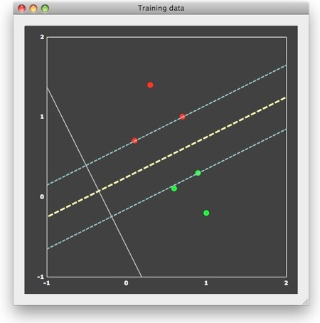
This "optimal" choice is intuitively clear and mathematically specified as large-margin separation. The "margin" is the distance of the separation line to the closest points of each class. The thin dashed lines in the figure above run in parallel to the decision boundary and indicate the end of the margin on both sides. According to the large-margin separation principle, a SVM selects the separating line producing the largest margin. Note that the resulting line would be the same even if the one red and one green point far away from the margin would not be present. In fact, the result would be the same even if there would be many additional points, as long as they would not fall within the margin. In other words, only the patterns at the margin determine or "support" the solution. Since mathematically each point is treated as a vector, these critical patterns are referred to as "support vectors".
A trained classifier is able to predict not only the class for the training patterns, but will also classify any new test pattern (generalization). The predicted class can be calculated using the linear discriminant function:
f(x) = wx + b
In this function, x refers to a training or test pattern, w is referred to as the weight vector and the value b as the bias term. The term wx refers to the dot product (inner product, scalar product), which calculates the sum of the products of vector components wixi. In case of two features, the discriminant function is, thus, simply:
f(x) = w1x1 + w2x2 + b
After training, the SVM provides us with estimates for w1, w2 and b. In the example, the weight value for feature 1 is "0.7", the one for feature 2 is "1.3" and the bias is "-0.2". The white line in the figure above visualizes the resulting discriminant function defined by these values. When evaluating this equation, the resulting sign divides the 2D space into two regions. The decision line can thus be constructed as the line, which crosses the discriminant function at the point where f(x) = wx + b = 0, and the dashed thin margin lines can be constructed as the lines crossing the discriminant function at the points where it evaluates to "-1" and "+1", respectively. When evaluating the discriminant function for a training pattern or a new test pattern, one actually projects the corresponding point onto the line defined by the disriminant function: if the projection falls on the positive side (y > 0), the pattern is classified as belonging to class 1, otherwise as belonging to class 2. While not exactly correct, the discriminant function can be interpreted as a line oriented in such a way that the resulting projection of points maximally separates the members of the two different classes (a parametric method more strictly based on this reasoning is Fisher's linear discriminant). For a linear classifier, the absolute value of the weights directly reflect the importance of a feature (voxel) in discriminating the two classes. In the example, the absolute value of weight 2 is larger (1.3) than the absolute value of weight 1 (0.7). While not as good as the discriminant function, feature 2 alone is able to separate the two classes (its values are the projections of the points onto the y axis), but not feature 1 (projections of the points on the x axis). This easy interpretation of the obtained weight values for linear classifiers allows to visualize them in a similar way as statistical maps (see below) and it allows to select the best features in case of a high-dimensional feature space.
Large-Margin Separation - The Soft Margin Case
Note that the large-margin separation principle is not only intuitive, but it is based in statistical learning theory due to the seminal work of Vapnik and collaborators relating the large-margin separation principle to optimal generalization performance. For linearly separable data, the SVM produces a discriminant function with the largest possible margin and since the decision line separates the two classes without error, it is referred to as the hard margin SVM. It can be shown that finding the maximal margin corresponds to solving an optimization problem, which involves minimizing the term ½||w||2 under the constraint that all exemplars are classified correctly. The term ||w|| refers to the norm or length of a vector, which is obtained as the square root of the scalar product of the weight vector with itself: ||w|| = sqrt(ww).
In practice, data is often not linearly separable; and even if it is, a greater margin with better generalization performance can be achieved by allowing the classifier to misclassify points (see below). The generalized SVM, which is able to handle non-separable data by allowing errors is referred to as the soft margin SVM. It involves minimizing the term:
½||w||2 + C Σξi
The new term on the right side sums over the (potential) errors produced for exemplars for a given weight vector. The ξi values are called slack variables; a slack variable is 0 in case of no error. If a pattern falls within the margin or even on the right side or on the other side of the decision boundary (miss-classification), the slack variable for this pattern is positive. The "cost" or "penalty" constant C > 0 is very important since it sets the relative importance of maximizing the margin and, thus, generalization performance (small C value) and minimizing the amount of classification errors (large C value).
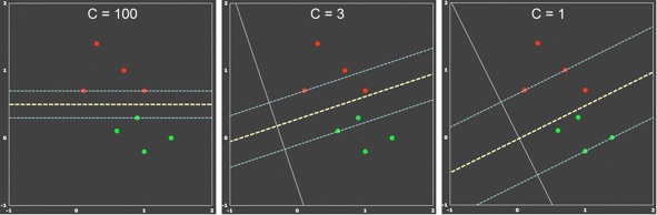
The figure above is an extension of example 1 where one point per class has been added. Although the data is linearly separable, it can be used to demonstrate the dependency of the soft-margin SVM on different C values. When C is large (left panel), the soft-margin SVM behaves as the hard-margin SVM. The resulting decision boundary leads to 100% correct classification of the training data, but the margin is small indicating sub-optimal generalization behavior. When the penalty value is reduced (C=3, middle panel), a larger margin is obtained at the cost that some points now fall within the margin. Reducing the penalty value even further (C=1, right panel) leads to an even larger margin. It is intuitively clear that the middle and right panels capture the underlying distribution of the data better and one would expect better generalization behavior than in the hard-margin case on the left side.
Cross-Validation and Model Selection
While the C parameter is very important, reasonable values will depend on the problem at hand. Which value should one choose? In machine learning terminology, specifying values for parameters such as C (as well as parameters for non-linear kernels) is referred to as model selection. Since the ultimate goal of training a classifier is to perform well on new data samples, one should test the generalization performance under different C values. When selecting the parameter C, one has to take care that this choice is made completely independent of the examples used for testing. An unbiased search for a good C value can be done by suitably splitting the data into several parts leaving one part aside for final performance testing. The reduced data set can be further split into a part for parameter optimization and a part for performance testing under different values. Instead of two completely separate parts, an often used technique to evaluate the performance of a selected parameter is n-fold cross validation. Using this technique, the training data is separated into several "folds" first. One fold is considered as the testing set and the other folds are used for training. Then the next fold is used for testing and all the others for training and so on. The average of accuracy on predicting the testing sets is the reported cross validation accuracy.
While one could just try out different C values and test their performance using n-fold cross-validation, a more systematic parameter search is usually applied. In this approach, the parameter (here C) is systematically changed in incremental steps over a sufficiently large range of values (e.g. 0.001 < C < 10000). For each parameter value, a cross-validation step is performed and the parameter value with the highest performance is finally chosen. The selected C value is then used to train the whole training data and the resulting SVM model is finally applied once to classify the separate test data. If class labels are available for the test data, one can then report the generalization performance of the classifier, e.g. the proportion of correctly classified test cases.
The next topic, Applying SVMs to ROIs. explains how the concepts described here can be applied to fMRI data sets from voxels in a region-of-interest (ROI). It will also be described how training and test patterns can be derived for ROIs from estimated single-trial responses and how the obtained SVM weight vector can be visualized using "VOM" files.
Note: BrainVoyager QX uses LIBSVM (see reference below) for training SVM classifiers.
References
Chih-Chung Chang and Chih-Jen Lin, LIBSVM: a library for support vector machines, 2001. Software available at http://www.csie.ntu.edu.tw/~cjlin/libsvm
COPYRIGHT
Copyright (c) 2000-2009 Chih-Chung Chang and Chih-Jen Lin
All rights reserved.

Redistribution and use in source and binary forms, with or without
modification, are permitted provided that the following conditions
are met:

1. Redistributions of source code must retain the above copyright
notice, this list of conditions and the following disclaimer.

2. Redistributions in binary form must reproduce the above copyright
notice, this list of conditions and the following disclaimer in the
documentation and/or other materials provided with the distribution.

3. Neither name of copyright holders nor the names of its contributors
may be used to endorse or promote products derived from this software
without specific prior written permission.

THIS SOFTWARE IS PROVIDED BY THE COPYRIGHT HOLDERS AND CONTRIBUTORS
``AS IS'' AND ANY EXPRESS OR IMPLIED WARRANTIES, INCLUDING, BUT NOT
LIMITED TO, THE IMPLIED WARRANTIES OF MERCHANTABILITY AND FITNESS FOR
A PARTICULAR PURPOSE ARE DISCLAIMED. IN NO EVENT SHALL THE REGENTS OR
CONTRIBUTORS BE LIABLE FOR ANY DIRECT, INDIRECT, INCIDENTAL, SPECIAL,
EXEMPLARY, OR CONSEQUENTIAL DAMAGES (INCLUDING, BUT NOT LIMITED TO,
PROCUREMENT OF SUBSTITUTE GOODS OR SERVICES; LOSS OF USE, DATA, OR
PROFITS; OR BUSINESS INTERRUPTION) HOWEVER CAUSED AND ON ANY THEORY OF
LIABILITY, WHETHER IN CONTRACT, STRICT LIABILITY, OR TORT (INCLUDING
NEGLIGENCE OR OTHERWISE) ARISING IN ANY WAY OUT OF THE USE OF THIS
SOFTWARE, EVEN IF ADVISED OF THE POSSIBILITY OF SUCH DAMAGE.
Copyright © 2023 Rainer Goebel. All rights reserved.