BrainVoyager v23.0
ANOVA with Two Within-Subjects and One Between-Subjects Factor
As an extension of the ANOVA with one within-subjects and one between-subjects factor, the ANOVA model described here allows to specify designs with two within-subjects factors and one between-subjects (grouping) factor. Different groups can be represented as levels of the between-subjects factor. The conditions applied to the subjects within each group can be represented as a two-factorial design if each subject received the same conditions (repeated measures). In the following, it is first described how to use the ANCOVA dialog to run the model over all voxels (or vertices) to obtain statistical random effects (RFX) volume or surface maps and how main and interaction effects as well as contrasts are tested. This is followed by a description how tabular data obtained from ROIs (or other sources) can be analyzied with this ANOVA model.
Providing a RFX-GLM as Input
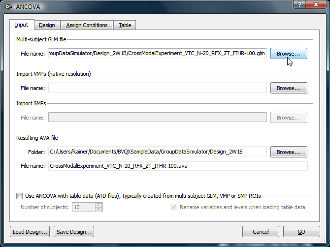
In order to run a ANOVA analysis for each voxel (or vertex) of volume (surface) data, open the ANCOVA dialog from the Analysis menu. If you continue right away from a computed RFX-GLM, the beta values are already available and the design can be specified in the displayed Design tab. If no appropriate GLM data structure is available, select a previously calculated RFX-GLM file in the Input tab (see snapshot below).
The program then switches automatically to the Design tab; in this tab the three-factorial design can be defined. The Design tab represents initially a design with one within-subjects factor, which is listed in the Factor list. The levels of this "Within 1" factor are shown in the Level list containing all conditions (names of beta values) found in the provided GLM file (see snapshot below).

Specification of the Design
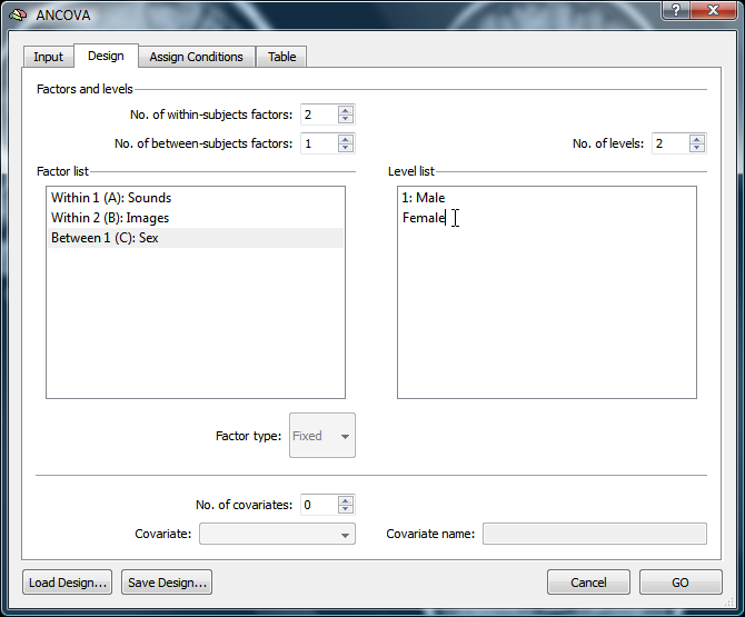
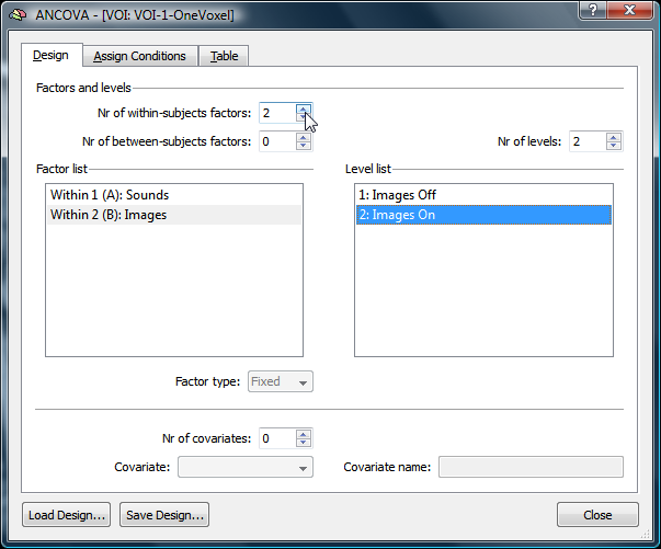
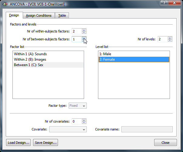
Since this model contains two within-subjects factors, add a second factor by increasing the value of the No. of within-subject factors spin box. This will add a second entry in the Factors list called "Within 2" as default. Since this ANOVA model also contains a between-subjects factor, the No. of between-subjects factors entry has to be set to value "1". This will add another entry ("Between 1") to the Factor list. In order to change the names of the three factors to reflect the design of the used example data, double click each factor name, which will activate text editing mode. After typing a name, click the return key or click somewhere outside the text field to leave text editing mode. The snapshot below shows the three names entered for the example data: "Sounds", "Images" and "Sex". Since each factor has two factor levels, change the No. of levels entry accordingly after selecting each factor in turn. Since the default number of levels is "2", only the number of levels for the first factor has to be changed in our example. Note that you can also remove a condition from the Level list by pressing the Delete key after highlighting an entry. To complete the specification of the design, also change the names of the levels for each factor; as with factor names, double click a level name to enter text editing mode.
It is useful to save the completed design to disk for later use (e.g. for applying it to ROI data, see below). Use the Save Design button to save the design as an ADS (ANCOVA design) file.
Since the number of factors and factor levels has been changed, the program may no longer know how the levels of the specified two within-subjects factors should be assigned to the variables found in the RFX-GLM file. This assignment can be performed in the Assign Conditions tab. For the case of two factors as in the example experiment, the Assign Conditions table (see snapshot below) shows four cells for each combination of the levels of the two within-subjects factors "Sounds" and "Images". In case that the levels of the two factors are named in such a way that their combination corresponds to the names of the variables in the GLM file, the assignment of cell levels to GLM variable names can be made automatically by clicking the Auto Assign button.
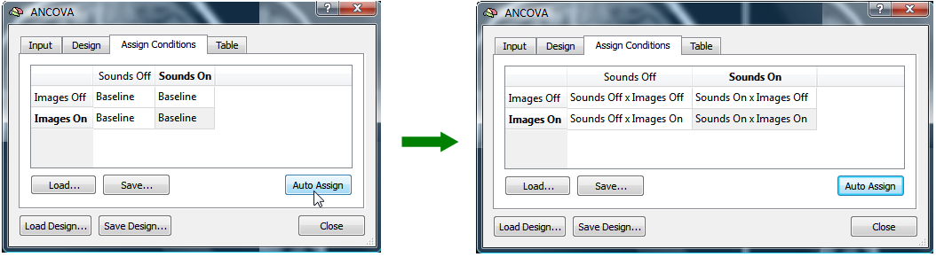
The resulting state of auto-assignment is shown on the right side in the snapshot above. In case that the assignment can not be performed automatically (i.e. if the naming of condition levels in the design does not match the naming in the GLM file), the assignment can be performed manually by double clicking each cell of the Assign Conditions table; this will open a list with all variable names found in the GLM file; in the example data, the names are "Baseline", "Sounds Off x Images Off", "Sounds On x Images Off" and so on.

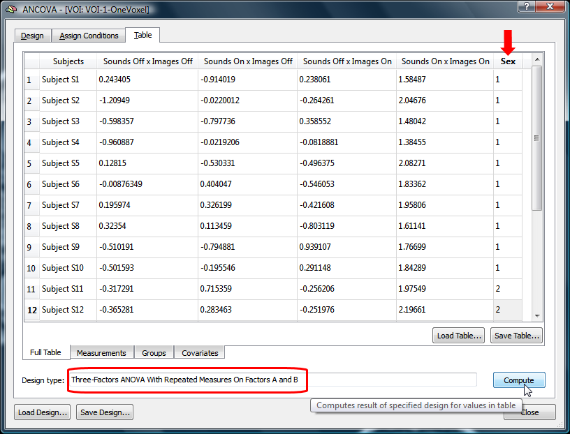
The final step before running the ANOVA is performed in the Table tab. The Design type field shows that a three-factorial design has been specified with two within-subjects factors (see snapshot above). Each row of the table contains cells for the data of a subject. The data for the four levels of the two-factorial within-subjects data are empty because the respective beta values are different for each voxel (or vertex). Furthermore, a column called "Sex" is shown on the right (see snapshot above), corresponding to the between-subjects (third) factor "Sex" with entries of "1" (level 1, "Male" group) and "2" (level 2, "Female" group). Note that the program assigns the first half of subjects into group 1 and the second half into group 2 as default, but this automatic assignment is probably not correct for your data! It is important that you specify the correct group assignment for a specific experiment by entering the correct level (group) value in the between-subjects factor column. You can also save a made group assignment to disk for later use independently from the content of other variables by clicking the Save GPA button in the Groups sub-tab. To finally run the ANOVA for all voxels (or vertices), click the GO button. As a result, an F map will be shown testing for the main effect of factor A ("Sounds" in the example).
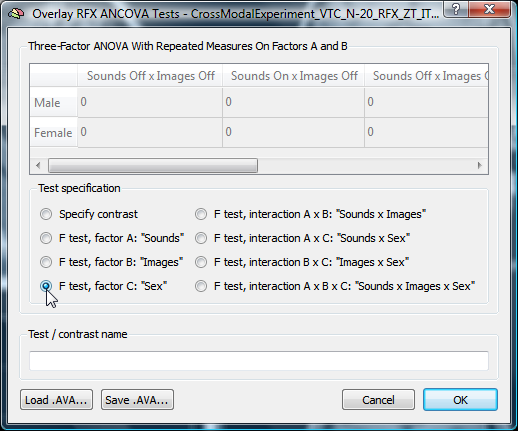
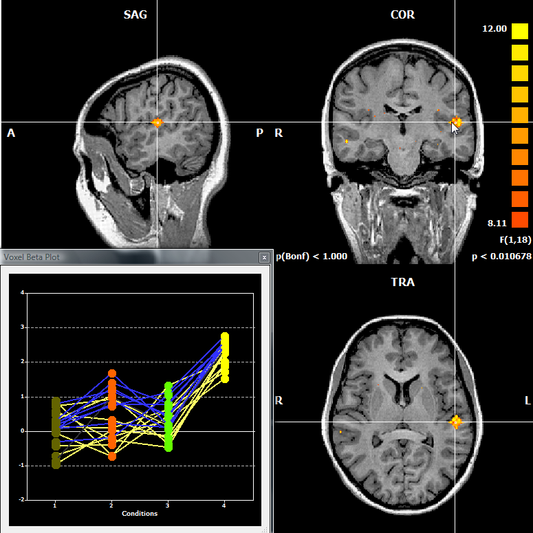
In order to test for specific main or interaction effects (F tests) or contrasts (t tests), the Overlay RFX ANCOVA dialog can be used, which can be launched by selecting the Overlay RFX ANCOVA entry in the Analysis menu. In the snapshot above an F test is selected testing for the between-subjects factor "Sex". The snapshot below shows the resulting F map with a region (simulated area "VOI 1") exhibiting a significant main effect of that factor (uncorrected for multiple comparisons). The mean difference between the "Male" and "Female" groups is also seen in the voxel beta plot (yellow lines indicate subjects of group 1, blue lines indicate subjects of group 2).
By re-entering the Overlay RFX ANCOVA dialog, other tests can be specified including contrasts. The Specify contrast options is selected as default. To specify a contrast click once or more times on a cell, which will change the values in the cell from "+1", "-1" to "0". For a valid contrast, the sum of the entered values must be "0".
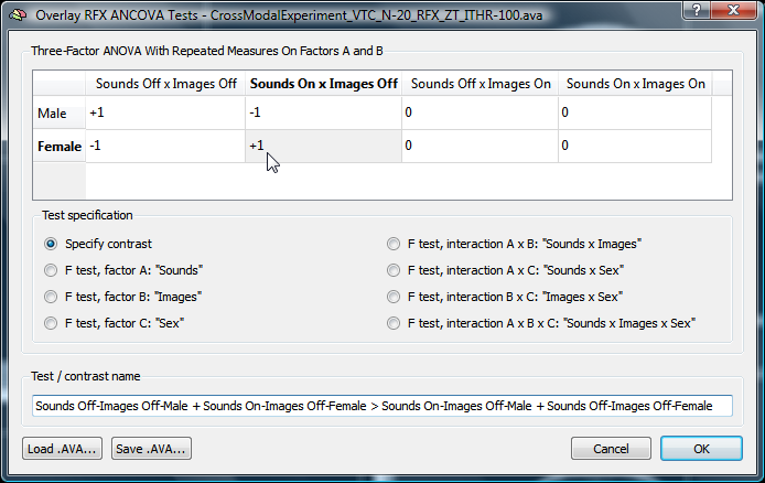
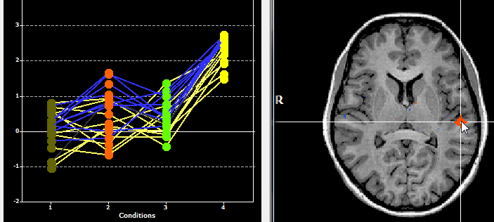
In the snapshot above, a contrast is specified for a specific interaction, which tests whether the effect of "Sound" is different for "Male" vs "Female" subjects in the "Images Off" conditions. The t map below shows that voxels in "VOI 1" (but not in "VOI 2") show a weak interaction effect, which can also be seen from the first two columns in the voxel beta plot
Three-Factorial ANOVA for ROI Data
Besides calculating statistical ANOVA maps (VMPs or SMPs), it is possible to run the ANOVA analysis for any region-of-interest (ROI) resulting in detailed numerical output (see below). The ROI-based analysis operates in two stages. First, a RFX GLM calculates beta estimates for all main conditions using the data (ROI time courses) of each subject. The estimated beta values per subject are extracted and saved in a ATD ("ANOVA table data") text file. This text file can then be loaded as input in the ANCOVA module and analyzed with an appropriate design.
NOTE: Separating the analysis in two stages has the advantage that the ANCOVA module can not only be used to analyze ROI-based data, but also data from other sources, e.g., behavioral data.
Step 1: Creating ANOVA Table Data by Estimating Subject-Specific Beta Values
As a prerequisite of ROI-based ANCOVA analysis, VOIs (or POIs) must be available, which can be loaded from disk or directly defined from functional or anatomical data. For the data used below, four VOIs have been defined. In order to calculate the beta estimates for each subject, open the VOI Analysis Options dialog, which itself can be called from the Volume-Of-Interest Analysis dialog. Select the ANCOVA tab to access the RFX-GLM functionality (see snapshot below).
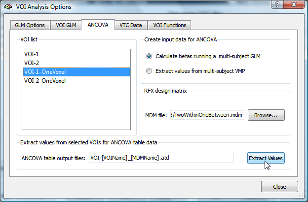
Select one (or more) VOIs from the VOI list. For each selected VOI, a resulting ATD text file will be created containing the beta estimates of all modeled main conditions per subject. In order to estimate the beta values, a multi-subject design matrix file has to be selected in the RFX design matrix field (here we use the "TwoWithinOneBetween.mdm" file, which was used above to calculate the whole-brain RFX-GLM). To start the generation of the ATD file, click the Extract Values button. This starts calculation of a first-level RFX-GLM over the VOI time courses for all subjects listed in the MDM file. The obtained VOI beta values are saved in a ATD text file with a name containing both the respective VOI name as well as the name of the chosen multi-subject design matrix (MDM) file as indicated in the ANCOVA table output files text field. For our example using VOI "VOI-1-OneVoxel" and MDM file "TwoWithinOneBetween.mdm", the resulting ATD file is named "VOI-VOI-1-OneVoxel_TwoWithinOneBetween.atd". The snapshot below shows its content.
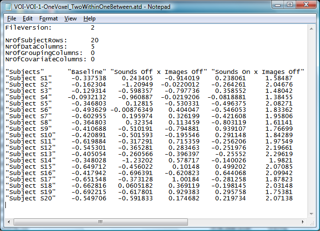
Since the example data contains 20 subjects, the main section of the file contains 20 rows with the estimated beta values. According to the setting stored in the MDM file, the ROI time courses may be z or percent-signal-change transformed before estimating the beta values; you may change the transformation type in the Time course normalization applied to each run field of the GLM Options tab prior to clicking the Extract Values button; in this example, z transformation has been used. Since the experiment uses a 2x2 factorial design within each subject, there are four betas estimated, each corresponding to one "cell" of the 2x2 desgin. As a fifth value (first column), the estimate of the baseline (value of constant after z normalization) is shown for each subject.
Step 2: Analysis of ANOVA Table Data
After creation of the ATD file containing the beta estimates per subject, the ANCOVA dialog is used to analyze the data with the desired model. In case that only one VOI file has been processed in the previous step, the ANCOVA dialog is started and the created ATD file is loaded automatically (see snapshot below). In other situations, the ANCOVA dialog may be called manually by clicking the ANCOVA Random Effects Analysis entry in the Analysis menu. In order to prepare the dialog for the analysis of table data, the Use ANCOVA with table data option must be checked in the appearing Input tab; you may also specify the number of subjects in the Number of subjects field, but this value will be adjusted when subsequently loading a ANOVA table data (ATD) file.
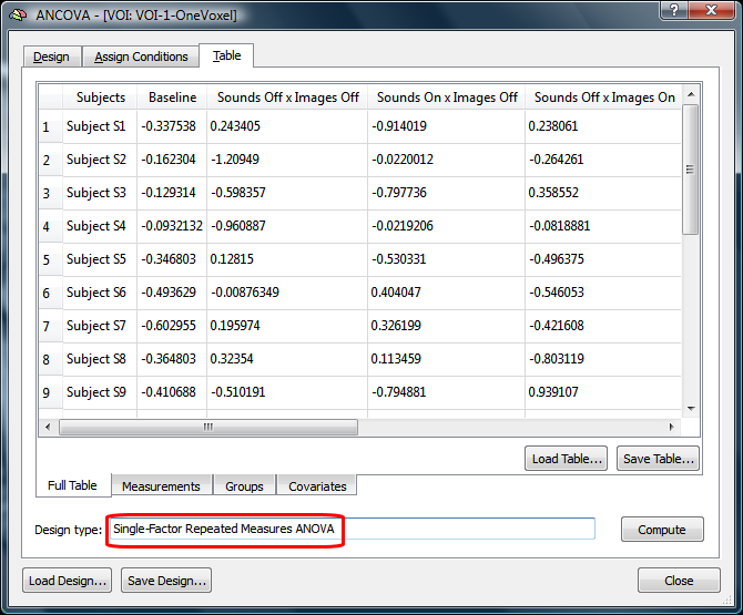
In case that the ANCOVA dialog is launched automatically after completion of step 1, it will show three tabs, the Design, Assign Conditions and Table tab; if the dialog is launched from the Analysis menu, it will also show the Input tab. After (automatically) loading the created ATD file, each row of the data in the Table tab are the estimated VOI beta values of a subject. As indicated before, the ANCOVA dialog assumes a single-factor repeated measures model as default. In order to analyze the data with the desired three-factorial model, the design must be changed by adding a second within-subjects factor as well as a between-subjects factor in the Design tab. A more convenient way to adjust the model is to reload the previously saved design specification (e.g. "Design_2W1B.ads") using the Load Design button. In the following, the manual adjustment of the design is explained.
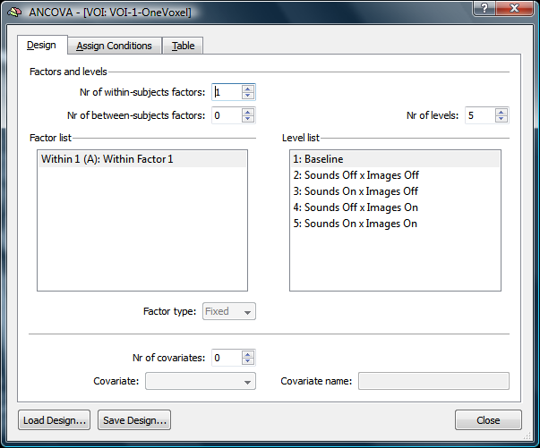
To adjust the model, the Design tab must be used. In our example all five conditions appear as levels of a single within-subjects factor. Since we need to specify two levels per factor, three conditions can be removed from the first factor either by clicking the Delete key after highlighting a condition or by reducing the Nr of levels entry to value "2". The two remaining levels should be renamed to correspond to the names of the two levels of the first within-subjects factor, which are "Sounds Off" and "Sounds On" for the example experiment (see snapshot below).
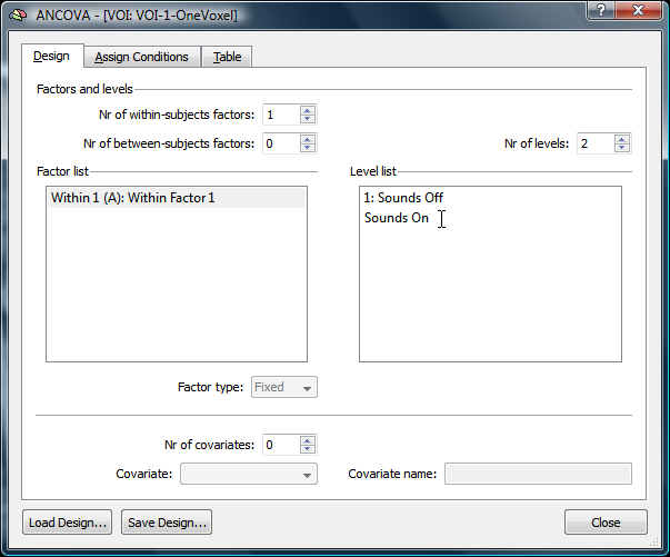
To change the name of a level or factor, simply double click the respective entry, which will enable text editing mode. When the new name has been entered, click the Return key or click outside of the text field to leave text editing mode. After changing the names of the two levels, also change the name of the first within-subjects factor (e.g. "Sounds").
As a next step, the second within-subjects factor can be added by increasing the No. of within-subjects factors entry to value "2" (see snapshot above). This will add factor "Within 2 (B)" in the Factor list (see snapshot above). Change the name of the second within-subjects factor to "Images" and the two levels of that factor in the Level list to "Images Off" and "Images On".
In order to complete the design, a between-subjects factor is added by setting the No. of between-subjects factors entry to value "1" (see snapshot above). According to the example data, the name of this factor is specified as "Sex" and the two levels of that factor are labeled as "Male" and "Female". The completed design specification can be saved to disk using the Save Design button.
Since the number of factors and factor levels has been changed, the program may no longer know how the columns of the loaded ATD file have to be assigned to the levels of the two within-factors. This assignment can be adjusted in the Assign Conditions tab. For the case of two factors as in the example experiment, the Assign Conditions table shows four cells for each combination of the levels of the two factors "Sounds" and "Images". In case that the combination of factor level names corresponds to the names of the columns in the data table, the assignment of cell levels to data columns can be made automatically by clicking the Auto Assign button. The resulting state of auto-assignment is shown on the right side. In case that the assignment is not performed (i.e. if the naming of condition levels in the design does not match the naming in the table data), the assignment can be performed manually by double clicking each cell of the Assign Conditions table; this will open a list with all variable names read from the ATD file; in the example data, the names are "Baseline", "Sounds Off x Images Off", "Sounds On x Images Off" and so on.
As opposed to the initial display, the Table tab now shows the correct model in the Design type field (see snapshot above). The table contains the beta values for all subjects from the ATD file, which we know are now assigned correctly to the four cells of the 2x2 within-subjects part of the design. Furthermore, a column called "Sex" is shown on the right (see snapshot above), corresponding to the between-subjects (third) factor "Sex" with entries of "1" (level 1, "Male" group) and "2" (level 2, "Female" group). Note that the program assigns the first half of subjects into group 1 and the second half into group 2 as default, but this assignment is probably not correct for your data! It is important that you check the assignment and enter the correct group assignment for a specific experiment by entering the correct level (group) value for each subject in the between-subjects factor column. Note that you can also save a performed group assignment to disk for later use independently from the content of other variables by clicking the Save GPA button in the Groups sub-tab.
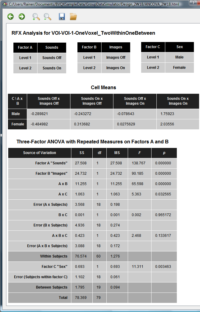
Clicking the Compute button will finally calculate the three-factorial ANOVA model for the data in the table. The produced output consists of three sections (see snapshot below). The first section describes the involved factors and their levels. The second section shows the mean values for each of the 8 cells (2 x 2 x 2 levels) of the three-factorial design. The third section shows the resulting ANOVA table with tests of significance for main and interaction effects. For the example data, all three factors exhibit a significant main effect. Also the interactions between the two within-subjects factors (AxB) and between the first within-subjects and the between-subjects factor (AxC) reach significance level.
Copyright © 2023 Rainer Goebel. All rights reserved.