BrainVoyager v23.0
ANOVA with One Within-Subjects and One Between-Subjects Factor
Many research questions require comparisons of several groups of subjects representing different populations. Examples of group comparisons are sex differences, multiple age groups, and patient groups. Different groups can be represented in the design described here as a between-subjects factor. The conditions applied to the subjects within each group can be represented as a within-subjects factor if each subject received the same conditions (repeated measures). In the following it is first described how to use the ANCOVA dialog to run the model over all voxels (or vertices) to obtain RFX statistical maps and how main and interaction effects as well as contrasts are tested. This is followed by a description how the ANCOVA dialog can be used to apply the one within-subjects, one between-subjects design to regions-of-interest (ROIs).
Providing a RFX-GLM as Input
In order to run an ANOVA analysis for this design, open the ANCOVA dialog from the Analysis menu. If you continue right away from a computed RFX-GLM, the beta values are already available and the design can be specified in the displayed Design tab. If no appropriate GLM data structure is available, select a previously calculated RFX-GLM file in the GLM / AVA tab. The program then switches automatically to the Design tab so that the two-factorial design can be defined. The Design tab represents initially a design with one within-subjects factor, which is listed in the Factor list. The levels of this "Within 1" factor are shown in the Level list containing all conditions (names of beta values) found in the provided GLM. The name of the within-subjects factor can be changed by editing the Factor name entry.
Specification of the Design
Since this model contains also a between-subjects factor, the Nr of between-subjects factors entry has to be set to value "1". This will add an entry ("Between 1") to the Factor list. To define the levels of the between-subjects factor, click on the "Between 1" entry in the Factor list. This updates several fields: The Factor name entry shows the current name for the selected factor, which can be edited (changed to "Sex" in the example snapshot below); the Nr of levels field shows the number of levels of the selected factor ("2" in the example below); the names of the factor levels are shown in the Level list. To change the name of a level, select a level in the Level list and then change its name in the Level name text box.
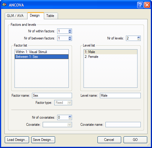
In the snapshot of the ANCOVA dialog above, example data of a simulated 2 factorial design is analyzed (for details, see online help of the Group Data Simulator plugin). The within-subjects factor is named "Visual Stimuli" and the between-subjects factor is named "Sex". The number of levels (default "2") of this factor needs not be changed since the design involves two levels. The names of the levels ("Level 1", "Level 2") are changed to the names of the study ("Male", "Sex").
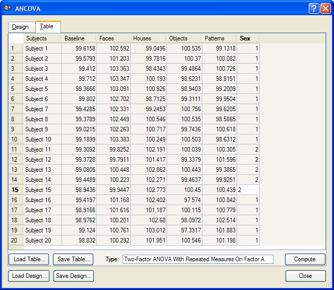
Assigning Subjects to Groups
Before running the ANOVA model, subjects have to be assigned to one of the groups, which is performed in the Table tab. This tab contains a table with placeholder entries for the voxel data for each subject. This table is filled with actual values if the dialog is used in the context of a ROI ANCOVA analysis (see below). When a statistical map is computed as in our case, the table is filled with "0" values. The last column of the table contains, however, the between-subjects factor ("Sex" in the example design) with values indicating to which group each subject is assigned to. Make sure that subjects 1 - 10 are assigned to level 1 (group "Male") and that subjects 11 - 20 are assigned to group 2 ("Female") by changing the default entries from "1" to "2" (or vice versa) for the respective subjects; while the default settings may sometimes match a given design, thie assignment must be carefully verified and modified if necessary. The specified design can be saved to disk by using the Save Design button (e.g. as "SimulatedVisualExperiment.ads"). To run the specified two-factorial ANOVA analysis, click the GO button. The resulting ANOVA results for each voxel are stored in the AVA file specified in the GLM / AVA tab.
Testing Effects and Contrasts
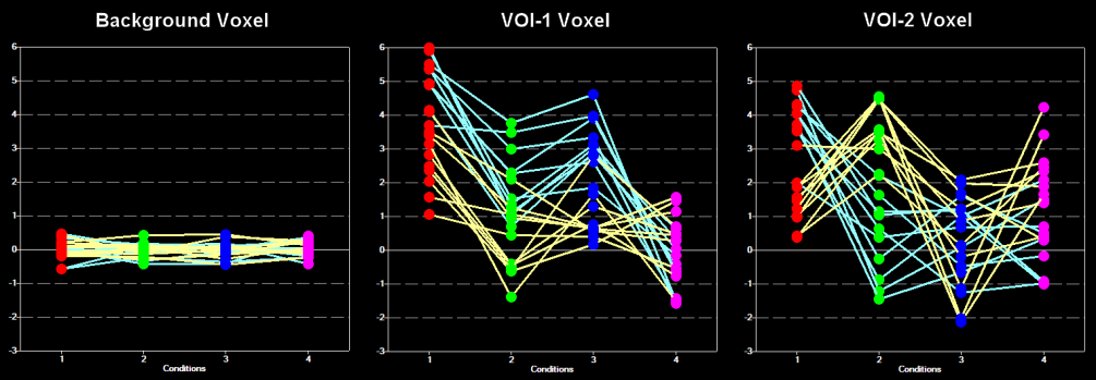
The two-factorial ANOVA model allows testing overall main effects for each factor as well as an interaction effect between the two factors. After calculating the model, an The two-factorial ANOVA model allows testing overall main effects for each factor as well as an interaction effect between the two factors. After calculating the model, an F map is shown as default testing significance of factor A (within-subjects factor "Visual Stimuli"). Other tests can be selected in the Overlay RFX ANCOVA Tests dialog, which can be invoked by selecting menu entry Overlay RFX ANCOVA in the in the Analysis menu. If this dialog is called and no AVA file is available, most options are disabled. In that case, the Load AVA button can be used to select the AVA file. The program tries also to load the original RFX-GLM file from which the AVA file has been calculated. While this GLM file is not necessary for overlaying ANOVA tests, it allows to show the Voxel Beta Plot dialog with the data (beta values) at the voxel under the mouse cursor. For the example data, the beta plot is shown above for three voxels, one from a "background" voxel, one from a voxel of "VOI 1" and one from a voxel of "VOI 2".
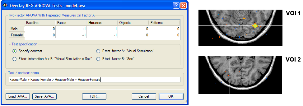
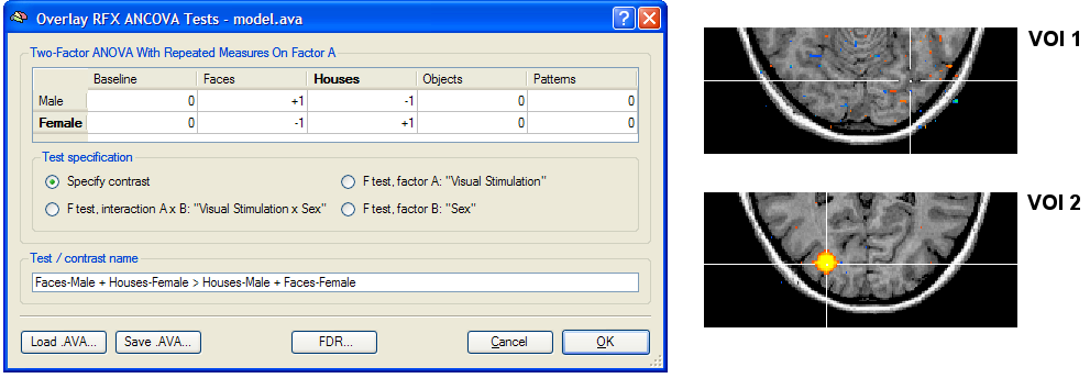
The Overlay RFX ANCOVA Tests dialog (see snapshot above) contains a contrast table showing the levels of factor A (within-subjects factor "Visual Stimuli" in the example design) in the top row and the levels of factor B (between-subjects factor "Sex") in the left column. The entries in the cells of the table can be changed to test specific contrasts comparing specific factor-level combinations. The options in the Test specification field allow to select the type of test, which can be a specific contrast (Specify contrast option, resulting in a t map), the F test for the within-subjects factor (F test, factor A option), the F test for the between-subjects factor (F test, factor B option) or the F test for the interaction between the two factors (F test, interaction A x B option). As default, multiple comparisons correction will be turned off for the resulting statistical (F or t) map but can be turned on using the FDR button. Clicking the OK button will calculate and overlay the selected test as a statistical map on the underlying anatomical data set (VMR or SRF). In the snapshot above and below a contrast test has been selected. The entries in the cells of the contrast table can be changed from "0" to "+1", "-1" and "0" by clicking repeatedly on a chosen cell. Double-clicking a cell allows entering a numerical value directly. The specified contrast in the snapshot above tests the same contrast ("[Faces] > [Houses]") in both groups. The resulting t map shows a strong effect in the ROI "VOI 1" but not in the ROI "VOI 2", which is evident in light of the respective voxel beta plots. The snapshot below shows how a specific interaction effect across groups can be tested. The chosen contrast tests whether the difference "[Faces] - [Houses]" is significantly different for the "Male" vs the "Female" group. The resulting t map shows no significant effect for "VOI 1" but a highly significant effect for "VOI 2" as one would predict from the respective voxel beta plots shown above.
Two-Factorial ANOVA for ROI Data
Besides calculating statistical ANOVA maps (VMPs or SMPs), it is possible to run the ANOVA analysis for any region-of-interest (ROI) resulting in detailed numerical output (see below). The ROI-based analysis operates in two stages. First, a RFX GLM calculates beta estimates for all main conditions using the data (ROI time courses) of each subject. The estimated beta values per subject are extracted and saved in a ATD ("ANOVA table data") text file. This text file can then be loaded as input in the ANCOVA module and analyzed with an appropriate design.
NOTE: Separating the analysis in two stages has the advantage that the ANCOVA module can not only be used to analyze ROI-based data, but also data from other sources, e.g., behavioral data.
As a prerequisite of ROI-based ANCOVA analysis, VOIs (or POIs) must be available, which can be loaded from disk or directly defined from functional or anatomical data. For the example below, two VOIs, "VOI 1" and "VOI 2", were defined (for details, see the documentation of the Group Data Simulator plugin). invoke the ANCOVA dialog from the VOI Analysis Options dialog, which itself can be called from the Volume-Of-Interest Analysis dialog. Before calling the ANCOVA dialog, the same multi-subject design matrix file (e.g. "SimulatedVisualExperiment.mdm") used to calculate the RFX-GLM has to be selected in the Design matrix file text box of the GLM Options tab. When running the ANOVA, the MDM design matrix file is used to run a first-level RFX-GLM over the VOI time courses of all subjects in order to obtain VOI beta values as input for the second-level ANOVA analysis. After specifying the MDM file, the ANCOVA dialog can be launched from the VOI GLM tab by clicking the ANCOVA button in the VOI RFX analysis field. The dialog will show two tabs, the Design and the Table tab. The table in the Table tab contains the estimated VOI beta values estimated by internally running a GLM over the VOI time course data of each subject. As described above, the default design (one within-subjects factor) has to be changed by adding a between-subjects factor ("Sex") in the Design tab. A more convenient solution is to reload the previously saved design specification (e.g. "SimulatedVisualExperiment.ads") using the Load Design button. While the loaded design will add the between-subjects factor "Sex", it will not assign the subjects to one of the available groups. As described above, this assignment can be done in the Table tab containing the group factor "Sex" with the two levels "1" ("male") and "2" ("female") in the right most column (see snapshot below). To specify that the subjects 11 - 20 belong to group 2, change the respective entries in the "Sex" column.
After subjects 11 - 20 have been assigned to group "2", the two-factorial ANOVA model can be calculated by clicking the Compute button. The results are presented in tabular form in three sections (see snapshot below). The first section defines the factors A and B by showing their names as well as the names of all levels. The second section, "Cell Means", shows the mean values for all factor-level combinations.
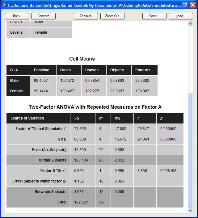
The third section shows the ANOVA table. The most important information of this table is the F test for factor A and B as well as the F test for the interaction between the two factors.
Validation of Calculations
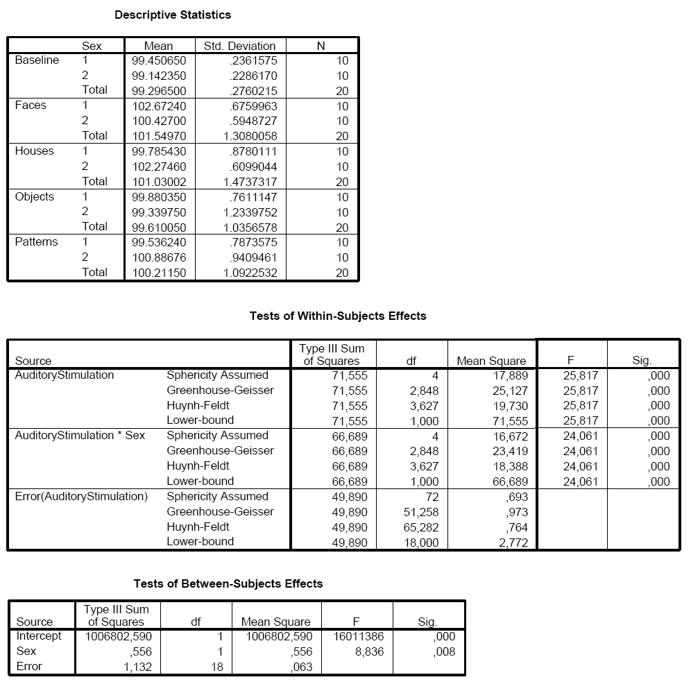
The VOI data of the table in the Table tab of the ANCOVA dialog can be saved to disk using the Save Table button allowing further analysis, if desired. During development of the ANCOVA module, the saved table data has been analyzed in SPSS 15 to test that the calculations in BrainVoyager are performed correctly. As the snapshot below shows, the results from the SPSS analysis are identical to the ones obtained in BrainVoyager. The "Descriptive Statistics" shows that the calculated mean values correspond to the values in section 2 ("Cell Means") of the BrainVoyager output. The SPSS results in section "Tests of Within-Subjects Effects" are identical to the results obtained for factor A and the interaction A x B in the BrainVoyager output. Finally, the SPSS results in section "Test of Between-Subjects Effects" are identical to the results obtained for factor B in the BrainVoyager output.
Copyright © 2023 Rainer Goebel. All rights reserved.