BrainVoyager v23.0
Whole-Mesh Cortical Depth Sampling
For standard resolution data (around 2 - 3 mm) it is appropriate to treat the cortex as a sheet without internal structure. For high-resolution (e.g. sub-millimeter) functional MRI data as obtained fom ultra high field scanners this assumption is too simplistic and very interesting data may be obtained from different cortical depth levels. The whole-mesh cortical depth sampling tool described in this topic can be used to sample high-resolution funcional data within grey matter (GM) at arbitrary relative depth levels. Since relative cortical depth sampling is built on top of cortical thickness evaluation, the method is based on the results of advanced segmentation and cortical thickness measurement tools. The VMR data set used for these tools should have high-quality with sub-millimeter (interpolated or measured) resolution, preferentially at 0.5 mm. Using the cortical thickness mesurement as input, a series of meshes is created at different relative depth levels from a starting mesh reconstructed at the surface running through the middle of the WM-GM and GM-CSF boundary. The created set of meshes at different cortical depth levels are then used to sample the functional data at the respective depth values. Based on the provided cortical thickness measurement, the reconstructed meshes follow the cortex at a constant relative depth level. The only issue of this approach is that the cortex is sampled based on the irregular spacing of vertex points of standard meshes. For even more precise depth sampling of small folded cortical regions, it is, thus, recommended to use the high-resolution grid sampling approach. While the result of cortical depth sampling roughly corresponds to sampling different cortical laminae, it is important to note that the relative position of laminae within the cortex depends to some extend on the curvature of the cortex, i.e. the relative position of a cortical layer is different at the fundus of a sulcus as compared to the crown of a gyrus. An optional (approximate) correction for this curvature-based lamina depth dependence is planned for a future release.
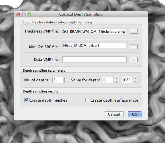
To start cortical depth mesh creation and sampling of functional data, open the Cortical Depth Sampling dialog by clicking the Cortical Depth Sampling item in the Meshes menu. The snapshot above shows the dialog on top of a mid-level grey matter mesh of the left hemisphere that was obtained as the result of cortical thickness measurement and subsequent application of the mid-GM volume creation procedure in the Mid-GM Volume tab of the Cortical Thickness Measurement dialog. The reconstructed border of this volume was loaded in the surface rendering window before opening the Cortical Depth Sampling dialog. The name of the reconstructed mesh ("Hires_MidGM_LH.srf") is shown in the Mid-GM SRF file text field. In case that the current mesh is not a mid-GM mesh, you can use the Browse ("...") button on the right side of the Mid-GM SRF file text field to select an appropriate mesh.
It is further necessary to select a cortical thickness map (VMP) file using the Browse ("...") button on the right side of the Thickness VMP file text field; the snapshot above shows part of the name selected for this example. The provided thickness VMP file is used to calculate relative depth levels for each vertex of the provided mid-GM mesh.
Creating Relative Cortical Depth Meshes
In case that the functional depth sampling step is not required, the dialog can now be used to create relative depth meshes in case that the Create depth meshes option in the Depth sampling results field is turned on (default). The number of desired depth meshes (default: 3) is specified in the No. of depths spin box in the Depth sampling parameters field. For each desired depth level a relative depth value can be provided in the right spin box of the Value for depth pair of spin boxes. Use the left spin box to select one of the relative depth meshes and enter a relative depth value in the right spin box. As default three relative depth meshes are specified with relative depth values of 0.25, 0.5 and 0.75. To create the specified meshes, click the GO button. The resulting meshes will be saved to disk with names indicating the relative depth level of the meshes. For the example above, the following 3 mesh files are stored to disk:
Hires_MidGM_LH_D-1-RD-0.25.srf
Hires_MidGM_LH_D-2-RD-0.5.srf
Hires_MidGM_LH_D-3-RD-0.75.srf
The end of the file names indicate the depth level ("D-[n]" part) and the corresponding relative depth level ("RD-[depth value]" part). The meshes are not loaded automatically, i.e. to visualize and use the meshes they need to be loaded as usual using the Load Mesh (and Add Mesh) items in the Meshes menu. The snapshot below shows the three loaded meshes each reconstructed at a different relative depth level.
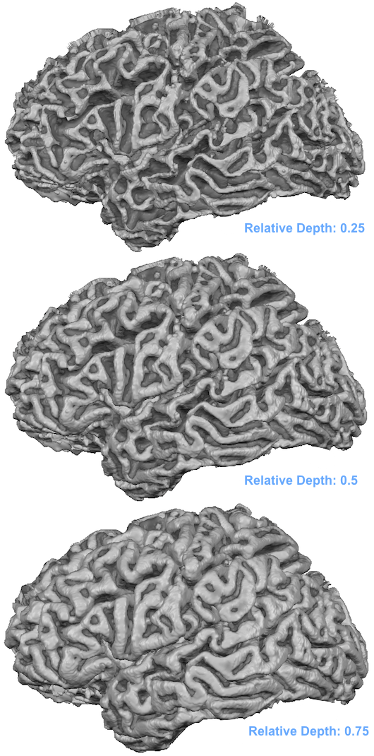
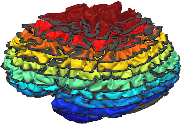
Note that the mesh reconstructed with relative depth level 0.5 looks not identical to the original mid-GM mesh. The reason is that the latter has been reconstructed in 0.5 mm voxel space, i.e. the resolution are increments of 0.5 mm whereas the 0.5 mm depth mesh may put a vertex at any fine-grained (float) value. While not necessary (and not recommended for functional data sampling), it might be useful for visualization to slighly smooth the created cortical depth meshes. Note, however, that smoothing may detoriate the precision of the reconstructed relative cortical depth level reflected in a mesh and should, thus, be done with care by only running a few smoothing iterations; furthermore it is recommended to use the curvature flow smooting method that is available in the Reconstructed Mesh Smoothing dialog since this smoothing approach minimizes geometric changes in the mesh. The snapshot below shows slightly smoothed versions of 10 meshes reconstructed at relative cortical depth levels of 0.05, 0,15 ... 0.95. The meshes were all loaded into one scene and sliced at different z levels to partially reveal all surfaces.
Sampling Functional Data at different Cortical Depth Levels
The created meshes can be used for MTC and SMP creation in the usual way using the Surface Maps and Mesh Time Courses dialogs; note, however, that the depth sampling "from" and "to" values in the Create MTC from VTC tab of the Mesh Time Courses dialog should be set both to 0.0 to restrict sampling to the position of the mesh vertices. In order to precisely sample analyzed functional data from high-resolution VMP data, the Cortical Depth Sampling dialog should be used. In addition to the mid-GM mesh file and the cortical thickness VMP file, this requires the additional specification of the (high resolution) VMP file containing the (statistical) map data. One way to obtain high-resolution VMP maps is to run GLM analyses using high-resolution (sub-millimeter) VTC data.
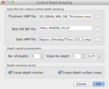
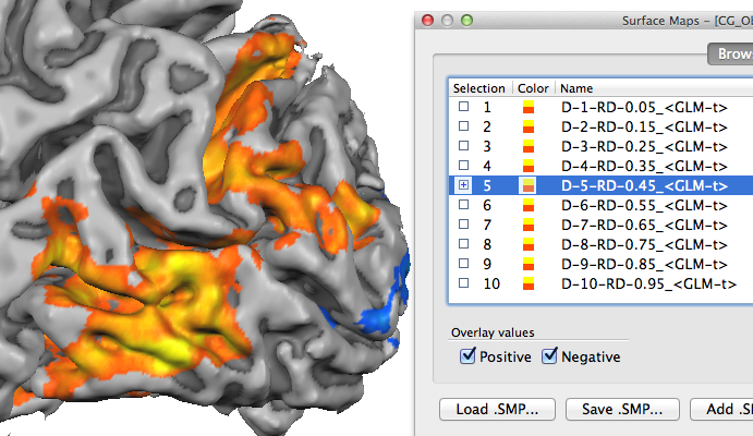
To specify an appropriate high-resolution VMP file, use the Browse ("...") button on the right side of the Data VMP file text box. As soon as a data VMP file has been specified, the Create depth surface maps option in the Depth sampling results field is turned on. When the GO button is clicked with this option turned on, the VMP file will be sampled at all requested cortical depth levels producing a set of surface sub-maps (see snapshot below). The names of the sub-maps indicate the depth level and relative depth value in the same way as described above for the saved mesh file names. In case that you want to create relative depth surface maps without explicit creation and storage of the respective meshes, turn off the Create depth meshes option before clicking the GO button.
Note. The depth level naming convention progresses from the white / grey matter boundary to the pial surface, i.e. a relative depth value of "0.0" corresponds to the WM-GM boundary and value "1.0" to the GM-CSF boundary. Since in the literature, e.g. in anaimal electrode recording studies, the opposite convention is often used, you may want to invert the relative depth values for publications or explicitly state that the relative depth values increase in the direction from the white / grey matter boundary to the pial surface.
Copyright © 2023 Rainer Goebel. All rights reserved.