BrainVoyager v23.0
Overlaying Volume Maps
Volume maps can be loaded and saved directly from the Volume Maps dialog. One of the most common ways to create volume maps is by running GLM analyses for single runs or for multiple runs including group GLM analyses. The snapshot below is the result of running a single-run GLM as described in the previous topic.
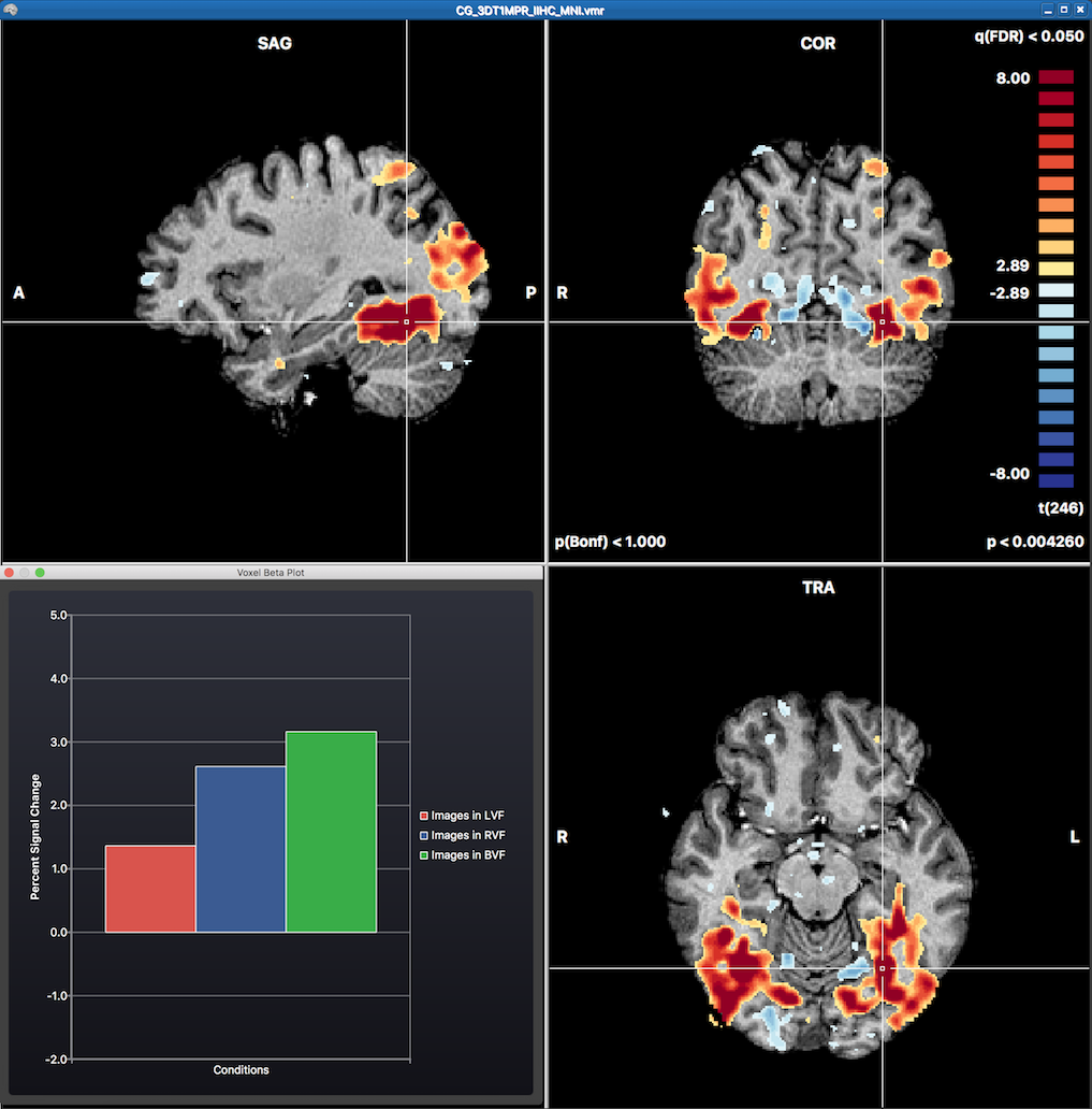
The statistical map can be explored in the VMR by moving the VMR cross through the three orthographic (sagittal, coronal, transversal) slice planes. Overlaying a statistical map will automatically also invoke the Voxel Beta Plot dialog in the left lower section of the VMR document window. This plot shows the beta values for the voxel under the current mouse cursor position (not the cross position). The initially displayed volume map after running a GLM is the result of the default contrast with all major conditions turned on (omnibus test). More specific contrasts can be specified using the Overlay GLM Contrasts dialog (see screenshot below).
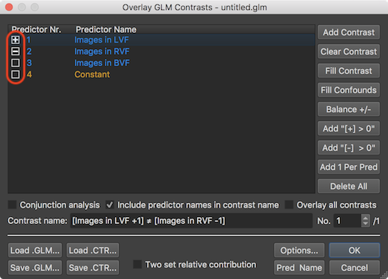
A specific contrast can be defined easily in the Overlay GLM Contrasts dialog by clicking inside the square boxes shown on the left side of each predictor displayed in the Predictor Name column of the GLM Predictor table. Clicking in an empty box will fill it with a plus sign indicating contrast weight value "1"; another click in the same box will fill it with a minus sign indicating contrast value "-1", and another click will make the box empty again indicating a contrast value of "0". In the snapshot above, the first predictor is filled with a plus, the second with a minus and the third is made empty, which implements the contrast "Images in LVF > Images in RVF" (if interpreted one-sided) or more genrally "Images in LVF ≠ Images in RVF". The name of this two-sided contrast is generated automatically and written in the Contrast name field together with the actual weight values. When now clicking the OK button, the specified contrast will be evaluated at each voxel using the beta values stored in the calculated GLM data structure. The contrast evaluation at each voxel results in a new parametric statistical t volume map that is overlaid over the anatomical document replacing the previously displayed volume map (see screenshot below).
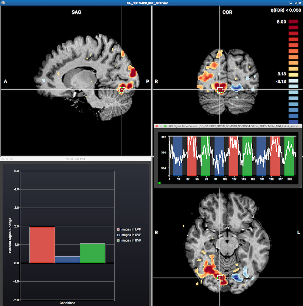
The snapshot above shows red colors in the right and blue colors in the left hemisphere corresponding to the expected results when contrasting visual stimulation in the left visual field ("Images in LVF") with stimulation in thre right visual field ("Images in RVF"). The mouse has been moved to the position of the cross revealing the fitted GLM beta values of the underlying voxel in the Voxel Beta Plot depicting a high value for the "Images in LVF" beta and a low value for the "Images in RVF" beta. Note that one can also invoke time course plot for any voxel or region around a voxel by CTRL-clicking (CMD-clicking on macOS) at a voxel. This has been done at the cross position revealing the respective time course of a region-of-interest (ROI) in the appearing ROI Signal Time Course dialog. Note that the height of the time course in the three main conditions matches the relative size of the predictors of the central voxel shown in the Voxel Beta Plot.
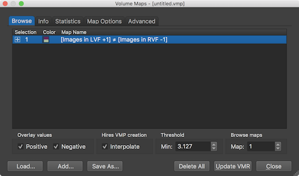
Properties of the displayed volume map(s) can be adjusted in the Volume Maps dialog. The Browse tab of the dialog (see screenshot above) shows a list of all currently available volume maps in the Maps table. The Map Name column shows the name of the map which can be changed by double-clicking it. When overlaying GLM contrasts, the name of the resulting map(s) correspond to the name of the contrast specified (automatically) in the Overlay GLM Contrasts dialog. A specific map can be included or excluded for the volume map overlay by checking or unchecking the respective map. A plus symbol in the Selection column indicates that the respective map will be visualized in the overlay, which is usually happening immediately but it can also be enforced by clicking the Update VMR button. Note that you do not have to click inside the square box to show/hide a specific map, it is sufficient to click anywhere inside the respective row of the Maps table. The Color column shows two colors from the chosen color look-up table used to display statistical supra-threshold (e.g. t values). If not changed in the Statistics tab, the default color look-up table (LUT) is used. The screenshots depicting the VMR document window with volume map overlays show the values of the default LUT visualized in a color bar. When both positive and negative values are enabled as in the example screenshots, the respective two halfs of the LUT are shown as a diverging color palette with the colors for minimum positive and minimum negative (threshold) values meeting in the center of the color bar (see screenshots above).
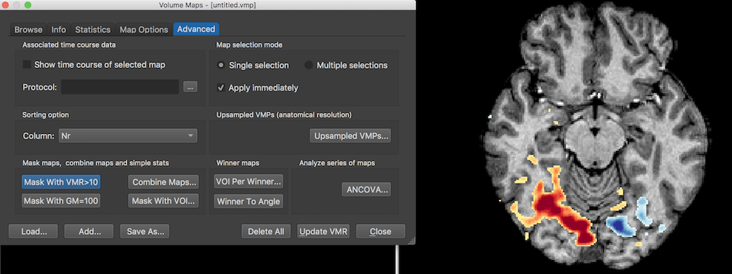
While the statistical map is corrected for multiple comparisions using BrainVoyager's default False Discovery Rate (FDR) approach, there is some noise activity outside the segmented brain volume. One can remove these clusters by clicking the Mask With VMR>10 button in the Advanced tab of the Volume Maps dialog. The screenshot above shows the result for the same axial slice shown in the screenshot above now without clusters outside the brain volume. The dialog also offers the option to mask the map with grey matter voxels by clicking the Mask With GM=100 button, but this should be used only if grey matter voxels have been set to a single value (100); such a VMR (ending in the substring "_WM_GM.vmr") is produced when running the advanced segmentation pipeline but it can also be approximated by using the "Range" tool in the Segmentation tab of the 3D Volume Tools dialog to map a range of grey matter intensity values (e.g. 60-120 in the example VMR data) to a value of 100.
Copyright © 2023 Rainer Goebel. All rights reserved.