BrainVoyager v23.0
Equi-Volume Depth Modelling
In the topic introducing regular grid sampling, grids were placed using an equidistant approach keeping a specified relative cortical depth level with respect to the cortex boundaries. For anatomical and functional data with very high spatial resolution (e.g. 0.5 mm iso-voxel data or better), the equi-distance sampling approach described in the previous topic will lead to misclassification of layers at regions of high curvature along the cortex (Waehnert et al., 2014). This is because layers seem to adjust their thickness to preserve layer-specific cortical volume (Bok, 1929). In order to more precisely assign voxels in the cortex to layer compartments, this principle should be used when sampling functional (or other types of) very high resolution data. Since BrainVoyager 20.4 an equi-volume sampling strategy can be selected both for regular grid and whole mesh depth sampling.
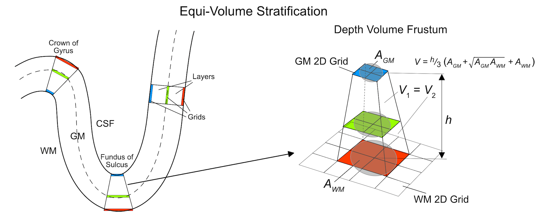
The figure above (Kemper et al., 2017) illustrates the principle of equi-volume cortical depth sampling for grids as implemented in BrainVoyager. The schematic explanation uses 3 grids and, correspondingly, 2 (big) layers filling the volume between the 2D grids. Equi-volume and equidistant sampling lead to the same depth sampling results in straight cortex (case of zero curvature shown on right side in left panel). The highest deviation from equidistant sampling occurs at the crowns of gyri and in the fundus of sulci since these regions have highest curvature. At the crowns of gyri (left upper case in left panel) the path for layers close to white matter along a cortex segment (e.g. blue grid) is much shorter than the path at the CSF (pial) border (e.g. red grid). To keep the volumes constant, layers need to move closer to the CSF border as is indicated for the green grid running through the middle of the cortex. At the fundus of sulci the situation is reversed, i.e. grids need to move closer to the white matter border in order to keep the volume of layers constant in a cortical segment (case at bottom in panel on the left).
The panel on the right in the figure above shows more details how grids are placed to meet the equi-volume criterion for the case of the fundus of a sulcus. Note that in case that grids are sampled using the Sample mid-GM grid and expand using streamlines option, the distances between grid points are squeezed and expanded in order to keep correspondence across the depth of the cortex automatically partioning the cortex in segments. When calculating the area A using the nearest neighbors of a corresponding position at different depth, the resulting area is larger in sections close to white matter (red rectangle in panel on right) and smaller in sections close to the CSF border (blue rectangle); in case of gyri, the opposite expansion and shrinking of areas across depth will be observed while in straight cortex the areas will have the same size. In ordet to adjust the position of a grid, the volume between grids within a section need to be calculated. The overall segment volume V can be approximated using the equation of a volume frustum. The volumes between grids, i.e. layers, can also be calculatd using the frustum equation. The position of vertices in the intermediate grids need to be adjusted according to desired relative depth levels in such a way that volume fractions relative to the overall volume of a segment remains constant. In the example above, the green grid nominally should run through the middle of the cortex implying to adjust the depth position in such a way that the two volumes V1 and V2 have the same volume fraction of 0.5 with respect to the overall segment volume. If this adjustment is performed for each segment, the resulting layers will exhibit a desired volume fraction throughout the extent of analyzed cortex.
Application
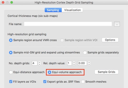
The Equi-volume approach option is turned on as default in the High-Resolution Cortex Depth Sampling dialog (see screenshot above). After loading an appropriate thickness map and specifying the region (via VOI or around 3D cross position) as described in the regular 2D grids topic, the equi-volume depth sampling approach, can be started by clicking the Sample Grids button. This will construct the regular grids at specified relative cortical depth levels - adjusted with respect to the equi-volume approach. As default, 4 grids will be created at the nominal depth values 0.0, 0.33, 0.66 and 1.0. The number of depth grids and their respective depth levels can be adjusted using the No. dpeth grids and Rel. depth value fields. For the example data shown in the screenshot below, the number of grids was changed to 5 with equally spaced nominal distances (depth values: 0.0, 0.25, 0.5, 0.75, 1.0).
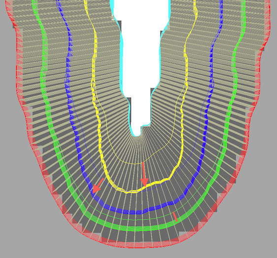
For demonstration purposes, the cortex depth sampling was run twice to create the screenshot above, once with equidistance and once with equi-volume sampling. The white lines running from the CSF boundary to grey matter indicate the established correspondence across depth used to partition the cortex in segments. As expected, grids close to the fundus of the depicted sulcus are pushed towards white matter and this effect decreases with increasing distance from the CSF boundary; the depicted red arrows (and red line) highlight the shift of the sampled grids for selected locations for the equidistant grid positions (thin yellow, blue, green lines) and for the equi-volume grid positions (thick yellow, blue, green partial grid meshes).
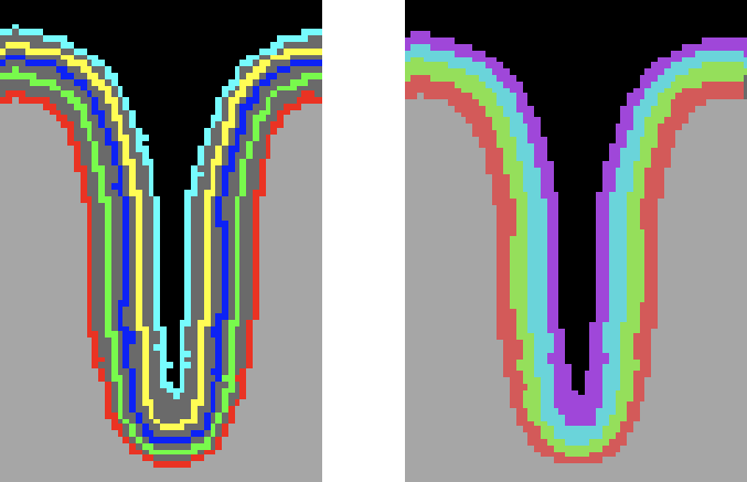
Knowing the coordinates of the equi-volume 2D grids is important for equi-volume depth modelling, but for sampling functional data from layer compartments the assignment of voxels to layers is of relevance. This assignment is performed in case that the Fill layers as VOIs option is selected (default) in the High-Resolution Cortex Depth Grid Sampling dialog. To perform the layer assignment, the signed Euclidean distance of each grey matter voxel to the grids in the neighborhood are computed allowing to determine the two gids enclosing the voxel. The following screenshot shows the grids as VOIs on the left side and the resulting colored layer VOIs after assigning voxels to layers (4) between grids (5).
Since each (colored) compartment is related to a layer-specific VOI, overlaid functional map or time course data can be selectively accessed using the standard VOI tools of BrainVoyager. The equi-volume cortex depth sampling tools are also available for the whole-mesh approach requiring a mid-GM mesh file next to the standard grey matter thickness VMP map as input. The Cortical Depth Sampling dialog can be invoked using the Cortical Depth Sampling item in the Meshes menu. The screenshot below highlights the options related to equi-volume and equidistance depth sampling options.
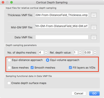
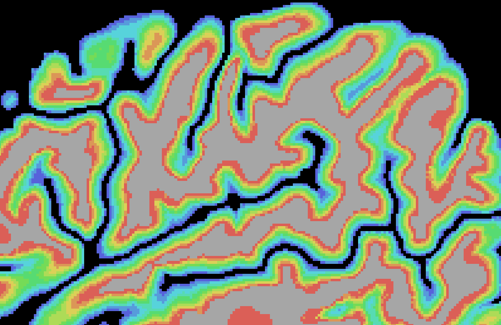
Like for the grid sampling approach, the equi-volume approach option and the Fill layers as VOIs option are turned on as default. It is also possible to smooth created depth meshes using the Smooth meshes option; this option uses the advanced smoothing that removes local high-frequency vertex fluctuations; this is, however, a rather slow process that needs to be applied for all depth meshes without changing the resulting meshes much, and it is thus recommended to turn it off. The screenshot below shows the result of the layer assignment process for an example data set using the whole-mesh equi-volume depth modelling approach with 10 layers (11 depth meshes).
Note that the created intermediate meshes can be saved to disk by turning on the the Save meshes option in the Cortical Depth Sampling dialog.
References
Bok, S.T. (1929). Der Einfluß der in den Furchen und Windungen auftretenden Krümmungen der Großhirnrinde auf die Rindenarchitektur. Zeitschrift für die gesamte Neurologie und Psychiatrie, 121, 682-750.
Waehnert, M.D., Dinse, J., Weiss, M., Streicher, M.N., Waehnert, P., Geyer, S., Turner, R., Bazin, P.L. (2014). Anatomically motivated modeling of cortical laminae. Neuroimage, 93, 210-220.
Kemper, V.G.,. De Martino, F., Emmerling, T.C., Yacoup, E., Goebel, R. (2018). High resolution data analysis strategies for mesoscale human functional MRI at 7 and 9.4 T. Neuroimage, 164, 48-58.
Copyright © 2023 Rainer Goebel. All rights reserved.