BrainVoyager v23.0
First-Level RSA
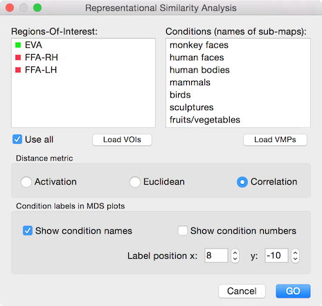
The goal of first-level representational similarity analysis (RSA) is to calculate the similarity of actvity patterns evoked by a set of conditions. The pairwise similarity measures between response patterns are stored and visualized in a representational distance matrix (RDM). The similarity between two condition response patterns is usually obtained by correlating the measured responses across voxels (spatial correction). Which voxels are used for calculating a correlation value is determined by one or more provided ROIs. As a preparatory step, a VOI file needs to be created containing all relevant ROIs, e.g. different brain regions relevant for a particular project. Note that one can define the set of VOIs for each subject individually (preferred) or by defining VOIs from a group map using the same group-ROIs for the data of individual subjects (not preferred since less powerful) from the same experiment. To analyze the data of a single subject with the Representational Similarity Analysis dialog (see snapshot above), the respective VOI file can be loaded in the dialog using the Load VOIs button. In the example represented above, three ROIs were previously defined for a single subject, one in early visual cortex, one in the left and one in the right (posterior) fusiform face area (FFA). If the Use all option is selected (default), RDM and MDS plots will be produced for all VOIs in the VOI List field. If one or more VOIs are selected, the Use all option will automatically turned off and the analysis is then performed only for the selected ROIs.
The estimated condition responses need to be provided as a set of volume maps stored in a VMP file, e.g. as the result from overlaying beta or t maps from a single or multi-run subject GLM analysis. The easiest way to produce this is to use the ... change condition names eventually. The Load VMPs button is used to load the desired VMP file. After loading the VMP file, the names of the sub-maps are listed in the Conditions List field. In the example represented above, a VMP file has been loaded containing 9 condition maps ("monkey faces", "human faces" and so on) estimated from a visual experiment.
The options in the Distance metric field can be used to specify which method to use for calculating (dis-)similarities between pairs of activity patterns. The Correlation option (default) calculates a Pearson correlation coefficient. The resulting r values ranging from -1.0 (perfect negative correlation) over 0.0 (no correlation) to +1.0 (perfect positive correlation) are transformed to a distance measure d by applying the equation:
d = 1 - r
The calculated d values, thus, fall in the range from 0.0 (minimum distance) to 2.0 (maximum distance) with value 1.0 in the middle representing no correlation. Note that the correlation calculated between patterns is sensitive to the similarity of the spatial patterns since this measure abstracts from the mean (and standard deviation) of the original values. Since this is a desired property, the correlation coefficient is used as default. It is also possible to calculate the Euclidean distance between pairs of activity patterns by selecting the Euclidean option in the Distance metric field. The resulting Euclidean distance values reflect, however, not only the similarity of distributed patterns but also the mean distance of the patterns. As a third approach, the Activation option can be selected that will only measure the paired distances between the spatial mean values of each condition. This measure, thus, reflects distances in evoked condition activation values as used in conventional ROI analysis. This measure is useful when contrasting it with the correlation measure to more clearly reveal whether the distributed patterns contain a different similarity structure than the one reflected in mean amplitude responses (see below for an example).
In addition to RDMs (one for each ROI), BrainVoyager also runs multi-dimensional scaling (MDS) on the distance values stored in the upper triangle of each RDM. The resulting MDS plots (one per RDM) visualizes the distances between conditions in a two-dimensional representation that greatly helps in appreciating the similarity structure coded in the RDMs. Note that if the analysis is repeated, different arrangements of the MDS items are obtained since distances are invariant with respect to (in-plane) rotation; furthermore, a truly multi-dimenstional (> 2) distance structure can not be projected uniquely into a two-dimensional distance space. Nonetheless, the resulting graphical display may greatly help in understanding the distance information encoded in the RDMs. For each item (condition) the MDS plot shows a point on the calculated 2D coordinates as well as a label identifying the item. The label is built from the condition names as shown in the Conditions List field in case that the Show condition names option is turned on in the Condition labels in MDS plots field. In addition to the condition name, a number identifying the condition as listed in the Conditions List field can also be shown in the item's label in case that the Show condition numbers option is selected. In order to save space (reducing overlap between labels), it might be also useful to only use condition numbers. The MDS item labels are shown next to the point visualizing the location of an item. The Label position x and Label position y value boxes can be used to change the relative position of the label with respect to the visualized point.
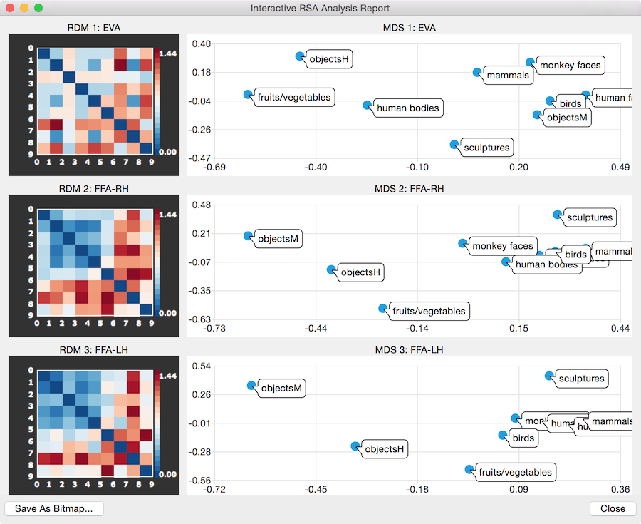
When clicking the GO button, a RDM and MDS output s calculated for each ROI and visualized in an Interactive RSA Analysis Report window (see snapshots above). The RDM and MDS plots belonging to each ROI are shown side-by-side, i.e. the RDM is on the left and the MDS plot is shown on the right side of the report window. For each ROI, such a RDM-MDS pair of plots is shown vertically from top to bottom. The report window can be resized to adjust the display to your needs and its content can be saved as a bitmap using the Save As Bitmap button. In case that more than 3-4 ROIs are analyzed, a scroll view window allows to move vertically through the plotted RDM-MDS pairs. For better comparison, the same maximum distance value is used in all individual plots to map the distance values to colors as opposed to using the maximum value of each RDM (an alternative way to aid in comparisons would be to percentile the distance values in each plot). Note that the report window is interactive, i.e. it is possible to click in each RDM plot to invoke the Matrix Plot Options dialog (see snapshot below) that can be used to change the maximum value used for color scaling in the Scale value box or to select another color look-up table than the default one using the Load LUT button.
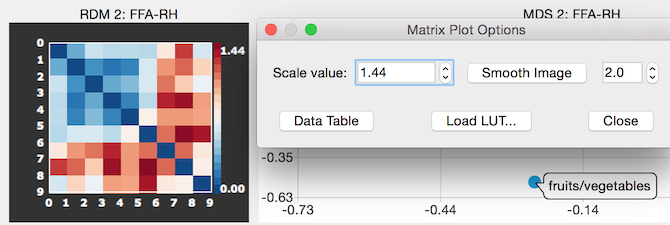
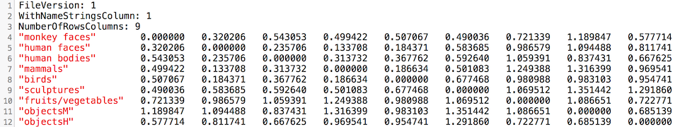
Clicking the Data Table button in the Matrix Plot Options dialog can be used to inspect the numerical distance values of the RDM. The values are also stored automatically for each RDM in a .rdm text file that can be used as input for seond-level RSA analysis. The .rdm file for the ROI FFA_RH of the used example is shown below.
The MDS plots are also interactive allowing to move the item labels to show occluded points or labels. The snapshot below is the same as above except that individual labels have been moved so that all 9 points and associated names are readable.
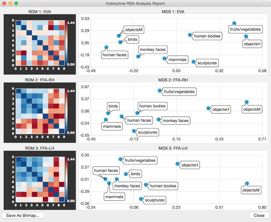
With the labels readable, it is now easy to see from the MDS plots that the two FFA RDMs represent very similar distance structures grouping all image responses from animate categories closely together separated from the responses to images from inanimate categories (the sculptures category is not that far away which is probably the case because they depict human body-like shapes). The similarity within the animate categories and their greater dissimilarity with the inanimate categories is also apparent in the RDM plots of the two FFA regions showing blue colors (small distances) in the left upper part (animate categories) and more orange/red colors (larger distances) in the other parts. The early visual area ROI (EVA) exhibits a less strong separation of the animate/inanimate category.
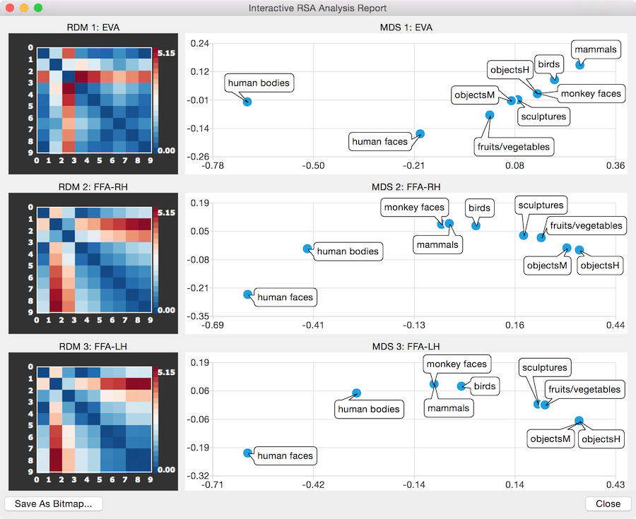
It is also instructive to compare the resulting RDM and MDS plots when using the activation distance metric (see snapshot above). In this case the MDS plot sorts the condition responses almost linearly (here roughly from left to right) with respect to the activation strength evoked by the different conditions; this solution is evident when inspecting the mean ROI responses of the three areas in a bar plot (see snapshot below).
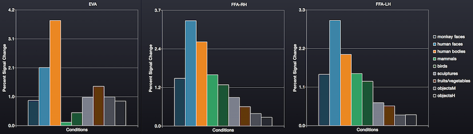
The comparison of the results when using the activation distance metric with the results when using the correlation metric reveals that the similarity between the distributed patterns reflects more high-level (semantic) information than the mean activation responses: while, for example, human and monkey images evoke very different response strengths in the two FFA regions, they are located close together in the correlation-based MDS plots.
Notes
Besides .rdm files, two .vom files are also created for each ROI when running the RSA analysis; these VOM files can be used for further analysis and visualization of the original activity patterns serving as input for the RDM calculation. The first .vom file (named "[ROI-Name].vom" contains the coordinates of the respective VOI in the native sapce of the functional data; the second .vom file (named "[ROI-Name]_Responses.vom" contains also the values (usually beta or t values) extracted from the provided .vmp file.
In the current version, only volume maps and volume ROIs can be used as input. It is planned to allow also surface maps (SMPs) and surface ROIs (POIs) as input in the next update of BrainVoyager.
Copyright © 2023 Rainer Goebel. All rights reserved.