BrainVoyager v23.0
EEG and MEG Inverse Modeling
Background
The linear discrete ECD model expresses the measurement m(t) from M channels as linear combinations of N dipolar source time-series s(t):
In (1) the columns of matrix A contain the lead fields of the dipolar sources for the given M-channel EEG/MEG configuration. si(t) = [sx(t), sy(t), sz(t)]t represents the source activity time-series of the current dipole placed on the i-th node of a mesh with N nodes and n(t) represents the channel noise.
All linear distributed inverse solutions can be expressed as a collection of many spatial filters (one per source dipole component and one per source position). Altogether, these spatial filters are applied to channel data for generating the estimated EEG/MEG source time-series in all source locations and for all source orientations
In this formulation, matrix W contains all spatial filter weights (one weight per source dipole component and location and per channel) and s(t) is the estimated source time-series for all components and locations. Assuming a measurement configuration with M channels, N sources and a free orientation model (i.e. X, Y and Z components are considered for each dipole), matrix W has order 3*NxM. If the orientation of each source is constrained (constrained orientation model), the order will be NxM. Similarly to the lead field matrix, the inverse solution matrix W is stored as a collection of 3*M or M maps (SMP) defined across all N source points depending on the orientation constrain.
The estimation of the inverse solution W in (2) can proceed by either attempting a total inversion of the distributed ECD model in (1) across the entire source space ("imaging" approach) or by filling three-by-three the rows of W at each source location ("scanning" approach).
The problem of all imaging approach is that N >> M, and this renders the linear problem (1) severely ill-posed, i.e. no unique solutions (1) exist if the only constrain is minimizing the residual term for fitting the measurements. Therefore, besides the obvious mathematical constrain or minimizing the residual term in (1), additional more "physical" constraints are to be posed to achieve a unique solution for (1).
One of the most popular "imaging" approach is the weighted minimum-norm (WMN). In this approach the weights in (2) are estimated in such a way to produce the source distribution with the minimum power that fits the measurements in a least-square-error sense:
Here, R represents the "a priori" source covariance matrix and is used to "inform" or "re-weight" the solution, i.e. to incorporate some prior knowledge about the spatial distribution of the source activity (R=I in case of no weighting). CN is the covariance matrix of the channel noise n(t) in (1) and is used to "regularize" the solution with respect to the actual noise distribution in the channel space (l is the regularization parameter controlling the amount of regularization in relation to the expected SNR, see below). CN=I corresponds to assuming the noise spatially uniform across all channel sites.
Since minimum-norm solutions are intrinsically biased towards superficial source locations, a typical weighting scheme called depth-weighting specifies R as a diagonal matrix with non-zero entries inversely proportional to the g-th power of lead field norms (g being the depth-weighting parameter):
An important variant of WMN is the Laplacian-weighted minimum norm which gives the mathematical basis of the so-called Low-Resolution Electro-magnetic Tomographic Analysis (LORETA) approach:
In (5) Vi represents the set of nearest "neighbors" of the source location at node (vertex) i on the grid (mesh) and Nmax the cardinal number of Vi. Rdw is the same as in (4) but allows combining depth- and laplacian- weighting.
Local Autoregressive Average (LAURA) weighting is similar to LORETA, but the physical distances between sources (nodes or vertices, dij) are involved in the weighting function and the cardinal number of Vi is allowed to vary across source locations:
Importantly, the diagonal WMN scheme in (4) can also be used for fMRI-constrained distributed inverse modeling by "modulating" the diagonal entries not only with the depth of the source with respect to the channels (depth-weighting), but also with local fMRI activity. For instance, BOLD percent signal change estimates (a) can be used to modulate by a flexibly variable amount (k=1, 2, ..., 10, ...) the diagonal entries of R that correspond to the locations of significant BOLD-fMRI activity (in the sense of a main effect vs baseline):
After estimation of the WMN spatial filter (3), some form of normalization of the weights is usually applied. Dale et al. (2000) have proposed scaling the filter weights at each source point to their variances in the channel space (noise-based normalization, NN). Applying the noise-based normalization has the important advantage of making the point-spread function of each source (i.e. the image of a point current source placed in a given position) more uniform across the entire cortical space, compared to the case of a minimum-norm solution without such normalization:
A variation of the noise-based normalization is the so-called standardized LORETA or s-LORETA (Pascual-Marqui et al. 2002) that normalizes the inverse solution at each source location using the so-called "resolution matrix" T. More specifically, the set of filter weights for the source at location i are jointly normalized using the i-th 3x3 block Ti along the diagonal of matrix T:
While weighting entails with applying data-independent mathematical and physical constraints to an inverse solution,a regularization parameter (lambda in equation 3) is also introduced to avoid magnification of errors in data in relation to signal-to-noise (SNR). In fact, due to the ill-posed nature of the problem of inverting the linear model in (1) for N > M, imaging approaches always requires some form of regularization. A convenient formula can be used to relate the regularization parameter to source SNR:
This formula allows adjusting the regularization in terms of a realistic guess for the signal-to-noise ratio (SNR) of the current sources. The higher the SNR guess in the formula (8), the lower the regularization parameter and more focal effects can be detected within that SNR range. Other effects at lower SNRs would still be detectable but only if occurring on more extended regions. A default value of 5 is realistic in many evoked response experiments.
Among the scanning approaches, a popular solution can be obtained using beamforming. The beamforming technique is a spatial filtering approach to source localization that can be thought of as being analogous to a frequency filter. In the same way as a frequency filter extracts those components of a signal containing some particular temporal characteristic, the beamformer spatial filter extracts the components of a signal with some specific spatial characteristic. Therefore, using beamforming it is possible to scan one by one each source location and retain a signal contribution that originates at that location in space while rejecting any contribution that originates at a different location. Using this principle, the subsets of weights in the matrix W corresponding to each specific source location (i.e. the triplets of rows of W) are estimated one by one from the data. Again, the channel data covariance C is used to this purpose. For instance, linearly constrained minimum variance (LCMV) beamformers (van Veen et al., 1997) use the following weight estimation for the source placed at location i:
Application
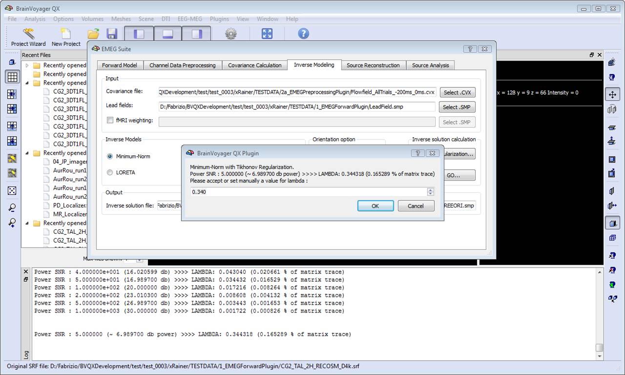
In order to estimate an EEG/MEG inverse solution to be used for source reconstruction and localization, it is necessary to switch to fourth tab of the EMEG suite dialog (Inverse Modeling). Starting from the lead field SMP estimated in the first tab and the covariance matrix estimated in the third tab, it is possible to estimate the inverse solution which will be again an SMP defined on the current mesh.
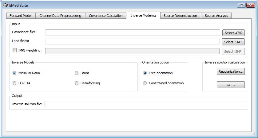
Regularization and normalization parameters can be set via the "Regularization ..." button. For all WMN solutions (Minimum-norm, LORETA and LAURA), a value can be specified for depth-weighting (see eq. 4), fMRI weighting (k in eq. 7) for the SNR guess (eq. 10). Please note: the lower the "guess" SNR the higher the value of lambda, which means less spatial resolution in change of higher sensitivity. The higher the "guess" SNR the lower the value of lambda which means higher resolution but lower sensitivity (i.e. we need higher SNRs to "resolve" a given source).
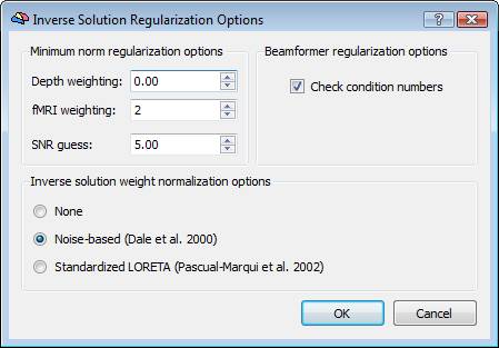
During progress, a number of guess SNR values are anyway displayed in the log tab to guide the user toward a possible different choice for SNR and lambda in a new estimation. Plotting the lambda values vs the SNR values would provide a typical L-shaped curve and one should choose the ideal "knee" of this so-called "L-curve". For each lambda value, the percentage of the trace of the "non-regularized matrix" is also reported. Normally these values should not go above 1% of the matrix trace, otherwise the resolution of the inverse solution becomes substantially worst.
References
Babiloni, F., Babiloni, C., Carducci, F., Romani, G. L., Rossini, P. M., Angelone, L. M., Cincotti, F. 2003. Multimodal integration of high-resolution EEG and functional magnetic resonance imaging data: a simulation study. Neuroimage. 19, 1-15.
Baillet, S., Mosher, J. C., Leahy, R. M., 2001.Electromagnetic Brain Mapping. IEEE Signal Processing Magazine 18, 14-30.
Brookes, M. J., Gibson, A. M., Hall, S. D., Furlong, P. L., Barnes, G. R. , Hillebrand, A., Singh K. D., Holliday, I. E., Francis, S. T., Morris, P. G., 2005. GLM-beamformer method demonstrates stationary field, alpha ERD and gamma ERS co-localisation with fMRI BOLD response in visual cortex. Neuroimage. 26, 302-308.
Brookes, M. J., Mullinger, K. J., Stevenson, C. M., Morris, P. G., Bowtell, R. 2008.Simultaneous EEG source localisation and artifact rejection during concurrent fMRI by means of spatial filtering. Neuroimage. 40, 1090-1104.
Dale, A. M., Sereno, M. I., 1993. Improved localization of cortical activity by combining EEG and MEG with MRI cortical surface reconstruction: a linear approach. J. Cogn. Neurosci. 5, 162-176.
Dale, A. M., Liu, A. K., Fischl, B. R., Buckner, R. L., Belliveau, J. W., Lewine, J. D., Halgren, E., 2000. Dynamic statistical parametric mapping: combining fMRI and MEG for high resolution imaging of cortical activity. Neuron 26, 55-67.
Darvas, F., Pantazis, D., Kucukaltun-Yildirim, E., Leahy, R.M., 2004.Mapping human brain function with MEG and EEG: methods and validation.NeuroImage 23, S289-S299.
Grave de Peralta, R., Murray, M. M., Michel, C. M., Martuzzi, R., Gonzalez Andino, S., 2004. Electrical neuroimaging based on biophysical constraints. Neuroimage 21, 527-539.
Hamalainen, M., Hari, R., Ilmoniemi, R., Knuutila, J., Lounasmaa, O., 1993. Magnetoencephalography - Theory, instrumentation, and application to non-invasive studies of the working human brain. Rev. Mod. Phys. 65, 413-497.
Hauk, O. 2004. Keep it simple: a case for using classical minimum norm estimation in the analysis of EEG and MEG data. Neuroimage. 21, 1612-1621.
Jeffs, B., Leahy, R., Singh, M., 1987.An evaluation of methods for neuromagnetic image reconstruction.IEEE Trans. Biomed. Eng. 34, 713-723.
Lin, F. H. , Witzel T., Hamalainen M. S., Dale A. M., Belliveau J. W., Stufflebeam S. M., 2004. Spectral spatiotemporal imaging of cortical oscillations and interactions in the human brain. Neuroimage. 23, 582-595.
Lin, F. H., Belliveau J. W., Dale A. M., Hamalainen M. S., 2006a. Distributed current estimates using cortical orientation constraints. Hum Brain Mapp. 27:1-13.
Lin, F. H., Witzel T., Ahlfors S. P., Stufflebeam S. M., Belliveau J. W., Hamalainen M. S., 2006b. Assessing and improving the spatial accuracy in MEG source localization by depth-weighted minimum-norm estimates. Neuroimage. 31, 160-171.
Pascual-Marqui, R. 2002. Standardized low resolution brain electromagnetic tomography (sLORETA): technical details. Methods Findings Exp Clin Pharmacol. 24, 5-12.
Pascual-Marqui, R., Michel, C., Lehman, D., 1994. Low resolution electromagnetic tomography: A new method for localizing electrical activity in the brain. Int. J. Psychophysiol. 18, 49-65.
Tikhonov, A., Arsenin, V., 1977.Solutions to ill-posed problems. Wiley, New York.
Copyright © 2023 Fabrizio Esposito and Rainer Goebel. All rights reserved.