BrainVoyager v23.0
Two-Factor ANOVA
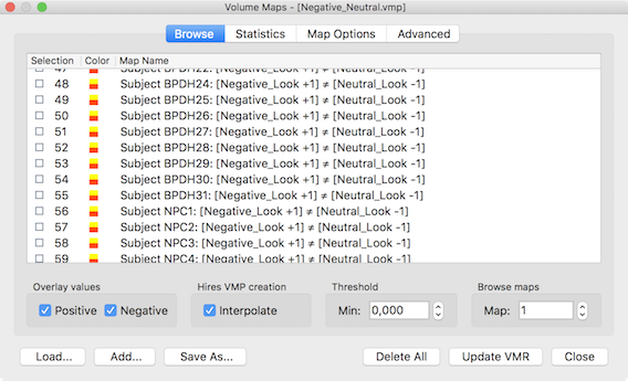
The two-way ANOVA model is an extension of the one-way ANOVA to two grouping factors where each item (i.e. scanned person) is grouped in two ways. Like the one factorial ANOVA, the model requires one continuous dependent variable as input that is analyzed with respect to two categorical between-subjects (grouping) factors, each with two or more levels (e.g. factor "disorder" with the levels "healthy participants", "disorder A", "disorder B", and factor "gender" with the two levels "male" and "female"). The model allows to analyze whether the two factors interact or whether they exhibit independent main effects on the dependent variable. In order to provide the dependent variable, it is recommended to create a VMP or SMP file containing one contrast map per subjerct as input. A GLM may also be provided but it is only possible to select one of the condition beta estimates as the dependent variable, i.e. you can (at present) not specify a ontrast when using the GLM as input. The snapshot below shows a VMP file with one entry per subject that has been prepared using the mentioned contrast map per subject tool in the Overlay GLM Options dialog.
Unbalanced Data
The between-subjects ANOVA model has been originally developed for balanced data, i.e. with an equal number of subjects assigned to each factor level combination, which are also called treatments. When data is unbalanced, there are different ways to calculate the sums of squares for ANOVA effects. There are at least 3 approaches, commonly called Type I, II and III sums of squares (introduced by the SAS statistics software). Which type to use has led to an ongoing controversy in the field of statistics (for an overview, see Heer (1986)). However, it essentially comes down to testing different hypotheses about the data. Note that when data is balanced, the factors are orthogonal, and types I, II and III all give the same results.
In a model with two factors A and B, there are two main effects, and an interaction, AB. The full model is usually represented by SS(A, B, AB). Other models are represented similarly: SS(A, B) indicates a model with no interaction, SS(B, AB) indicates a model that does not account for effects from factor A, and so on. The influence of particular factors (including interactions) can be tested by examining the differences between models. For example, to determine the presence of an interaction effect, an F-test of the models SS(A, B, AB) and the no-interaction model SS(A, B) would be carried out.
The Type I model tests one effect after other effects, i.e. first it tests the effect of factor A (SS(A)), then factor B (SS(A, B) - SS(A)), and then the interaction (SS(A, B, AB) - SS(A, B)). This sequential sums of squares calculation leads to different results depending on the order of the main effects. It can be shown that this approach is testing the first factor without controlling for the other factor. Because of these undesired properties, the Type I model is not used in BrainVoyager.
The Type II model tests for each main effect after the other, i.e. it tests the effect of factor A as SS(A, B) - SS(B), and the effect of factor B as SS(A, B) - SS(B). While this leads to results that are independent of the order of factors, this approach assumes that there are no significant interaction effects. Since this assumption is too limited for massive voxel-level testing, this approach is also not used in BrainVoyager (but it might be added as an option for ROI analyses in the future since it is more powerful than the type III model in case of no significant interaction).
The Type III model tests for a main effect after the other factor and interaction, i.e. the effect of factor A is tested using the difference SS(A, B, AB) - SS(B, AB) and factor B is tested as SS(A, B, AB) - SS(A, AB). This approach is, thus, valid in the presence of significant interaction AB. It should be noted, however, that it is often not interesting to interpret a main effect if interactions are present. Because of its least restrictive assumptions, the Type III model is used In BrainVoyager.
In the following, the two-factor ANOVA is demonstrated first using a whole-brain analysis followed by a region-of-interest analysis. The data used is from a study by Zutphen et al. (2016).
Specification of the Design
When providing a prepared VMP (or SMP) with one dependent variabler as input in the Import VMPs field, the dialog initially selects a one-factorial between-subjects design. In order to specify that a two-factorial design is desired, increase the No. of between-subjects factors spin box to 2 (see dialog below).
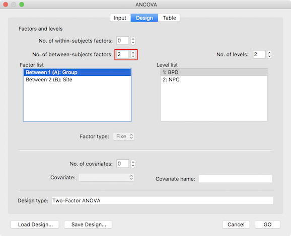
Furthermore, the names of the two factors can be changed to reflect the respective design by double-clicking the default name in the Factor list box; in the example used to illustrate the two-factor ANOVA, the two factors are labelled as "Group" and "Site". The levels for a selected factor are shown in the Level list box and the number and names of the levels can be adjusted by using the No. of levels spin box and by clicking on the default names in the Levels list box, respectively. In the example, the first factor (selected in the screenshot above) has two levels "BPD" and "NPC" representing a patient and control group and the levels of the second factor represent different scanning sites. It is recommended to save the specified design with factor and level neames to disk for later use (e.g. VOI analysis) using the Save Design button.
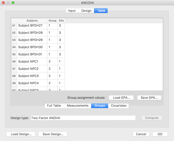
The final step before running the two-factor ANOVA model is to assign the subjects to the respective group cells (factor level combinations). This can be achieved using the entries shown in the Table tab (see screenshot above). While one can enter the grouping in the Full Table mode, for purely between-subjects designs it is more convenient to select the Groups tab, which restricts the table to the grouping assignment column(s) and allows to save/load grouping information in grouping (.GPA) files. The grouping sub-table shows two columns representing the two factors of the specified design. The cells need to be filled with level values starting with value 1 for the first factor level. The entries in a row for the two factors specify the level combination (cell) to which the corresponding participant will be assigned. The table in the snapshot above shows 51-59 of the full (97) participant list; subjects 51-55 are assigned to the cell [1, 3], which corresponds to the level combination "BPD" - "Luebeck" (borderline patient group, measured at site Luebeck) while subjects 56-59 are assigned to the group [2, 1], which corresponds to the level combination "NPC" - "Maastricht" (non-patient control group measured at site Maastricht). While it is recommended to assign the same number of subjects to each cell (balanced design), the subsequent analysis handles also unbalanced designes (see explanation above). After completing the grouping assignment, it is recommended to save the information to disk for later use using the Save GPA button. The whole-brain two-factor ANOVA can now be started by clicking the GO button.
Inspecting Two-Factor ANOVA Map Results
After running the two-factor ANOVA, a statistical map is shown testing for the effect of the first factor ("Group" in the example data). The F map for the first factor of the example data is shown in the screenshot below.
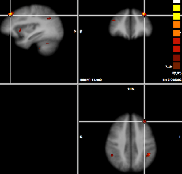
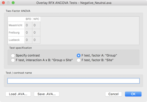
In order to test other effects of interest, the Overlay RFX ANCOVA Tests dialog can be invoked from the Analysis menu (or from the context menu of the VMR document). For two-factor ANOVA designs, the dialog offers testing for the main effect of factor A (resulting F map shown in the screenshot above for the example data), testing for the main effect of factor B and testing for the interaction between the two factos (see snapshot below). These tests can be selected by chedking the F test, factor A, F test factor B and F test, interaction A x B items followed by clicking the OK button.
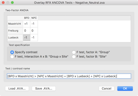
Besides these F tests, specific contrasts can be tested by selecting the Specify contrast option. After selecting this option, the contrast table in the upper part of the dialog will be enabled and the desired contrast can be entered by clicking into the cells repeatedly to cycle through the contrast values +1, -1 and 0. Other contrast values can be entered by double-clicking the cell to bring up a text editing field allowing to enter a number. Note that contrasts need to follow the typical rules of ANOVA models as described in standard statistical text books. In the example below, a contrast is entered testing for the main effect of patient vs control group but leaving out one scanning site.
ROI Analysis
The data from regions-of-interest (ROIs, i.e. VOIs in volume space and POIs in cortex surface space) are analyzed in the same way as for other designs. The only difference is that a two-factor ANOVA model needs to be specified and data from desired ROIs needs to be available. In order to avoid circularity, the ROIs should be determined from independent data, e.g. from anatomical coordinates or better from additioal functional localizers. It is usually also acceptable to use ROIs from the same data as long as the subsequent contrasts are not biased by the contrast used to select the ROIs (i.e. the subsequent contrasts need to be orthogonal to the selecting contrasts).
While the dependent measures can be manually entered (one value per subject), they can be also loaded from specific file types (".ATD" and ".DPV"). Both the VOI Analysis Options and the Patch-Of-Interest Analysis Options dialog contain routines to save data from multi-subject GLMs / VMPs and SMPs in ".ATD" ("ATD = ANCOVA table data) format, which can be read directly into the ANCOVA dialog. To start a ROI ANOVA analysis, the Use ANCOVA with table data option has to be checked in the Input tab of the ANCOVA dialog. While the number of subjects might be determined directly from a .ATD file later, it is recommended to also specify the number of subjects to analyze in the Number of subjects field.
For convenience, the ANCOVA dialog is opened and prepared for analysis when exporting ROI values from the VOI Analysis Options dialog that can be invoked by clicking the Options button in the Volume-Of-Interest Analysis dialog. In the screenshot below, a previously defined VOI ("Insular RH") has been loaded that is now available for subject-specific value extraction. Since we want to read the values from the previously prepared multi-subject VMP file, the Extract values from multi-subject VMP option need to be selected in the Create input data for ANCOVA field (see screenshot below).
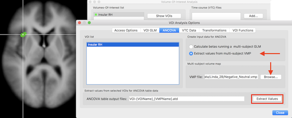
In case that the multi-subject VMP file (usually the same used also for the whole-brain analysis) has been already loaded in the Volume Maps dialog, the VMP file entry will automatically be filled with the respective file name. In case that the VMP file has not been already loaded, it can be done using the Browse button next to the VMP file text field. The Extract Values button can now be clicked in order to extract the subject-specific values from the specified VOI. The extracted data is not only saved to disk but also directly loaded into the ANCOVA dialog (see snapshot below).
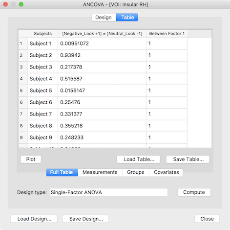
The presented ANCOVA dialog shows in the second column the extracted values per subject as desired but the default model and group assignment is not yet correct. While the design can be adjusted manually, it is easier to reload the design created and saved for the whole-brain analysis (see above), which will change the default model to a two-factor model and sets the factor and level names. In case that the grouping values for the third (factor A) and fourth column (factor B) were also saved earlier they can be loaded by switching to the Groups tab and using the Load GPA button. The prepared data table for a two-factorial ROI ANOVA looks than similar to the one shown below.
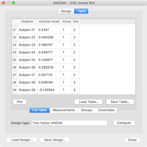
After clicking the Compute button, the ANOVA results are presented in a window and also saved to disk as a HTML file. The output first presents a title indicating the name of the ROI from which the data was extracted (see snapshot below). This is followed by two tables indicating the name and levels of factor A and factor B. The next table shows the cell means containing the average value of the dependent variable for each group (factor-level combination) as well as row/column values showing the factor level values averaged across all levels of the other factor respectively. The numbers in brackets next to each entry indicate the number of subjects assigned to each group. As you can see in the example output below, the study has a rather unbalanced design but can be analyzed using the Type III sums-of-squares model as described above. The ANOVA table is shown below the cell means presenting the results of testing for main effects (factor A, factor B) and/or the interaction effect between A and B.
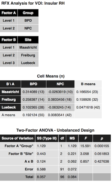
In the example data, the insular ROI data shows a highly significant main effect "Group", a nearly significant main effect "Site" and no interaction effect. Below the Two-Factor ANOVA table, critical minimal distances between cell means are shown that maybe helpful in case of more than two levels in order to decide which cells differ significantly from each other.
References
Herr DG (1986). On the History of ANOVA in Unbalanced, Factorial Designs: The First 30 Years. The American Statistician, 40(4), 265-270.
Zutphen L et al. (2016).
Copyright © 2023 Rainer Goebel. All rights reserved.