BrainVoyager v23.0
Single-Factor ANCOVA
In this model a single-factor ANOVA model is extended by specifying one or more additional continuous (quantitative) variables called covariates. The resulting single-factor analysis of covariance (ANCOVA) model explains variation in a dependent variable by combining a categorical (qualitative) independent variable with one or more continuous (quantitative) variables. If a covariate is linearly related to the dependent variable, it will reduce pre-existing variability between subjects. In effect, the variance component in the dependent variable which is due to covariation with the covariate is removed ("partialed out") from the dependent variable. This reduces the variance of the error term in the model, which increases the sensitivity of the ANCOVA as compared to the same model without the covariate (ANOVA model). A higher test sensitivity means that smaller mean differences between groups will become significant as compared to a standard ANOVA model.
Note that ANCOVA has a similar goal as repeated measures ANOVA, namely to remove pre-existing differences between subjects. In repeated measures ANOVA models, this is achieved by measuring the same subjects under various conditions (within-subjects) instead of assigning different subjects to different conditions. From the obtained data, changes of the dependent variable across conditions are only analyzed within each subject completely removing between-subjects variability. In ANCOVA models, the reduction of inter-subject variability depends on the strength of correlation of the covariate with the dependent variable. This consideration implies that ANCOVA models are only useful for designs with between-subjects factors but provide no benefits in pure within-subjects factorial designs.
Input Requirements
The single-factor ANCOVA accepts a multi-subject VMP or SMP file as input. A multi-subject GLM (e.g. RFX-GLM) can also be used but requires that a single value (beta) from repeated measures is selected as the dependen variable (currently no contrast can be specified in case a GLM is used as input). For fMRI data it is advised to first create a VMP/SMP from a multi-subject GLM by specifying any desired contrast (see below). Typical examples of covariance analysis are comparisons of fractional anisotropy (FA) maps between groups of subjects (multi-subject VMP) or comparison of cortical thickness maps between groups (multi-subject SMP). If differences in such dependent variables (FA, cortical thickness) are compared in several groups (e.g. one or more patient groups and a group of healthy controls), it might be very useful to aim to eliminate the effect of covariates such as age from the measurements. By removing the effect of a covariate (e.g. age, IQ), ANCOVA would allow to study group effects as if all subjects would have the same value of the covariate (e.g. same age, same IQ). The goal of the covariate can thus also be interpreted as adjusting the dependent measures in such a way that the subjects in the different groups have the same "starting condition" with respect to the controlled variable (e.g. age, IQ). Besides the value for the dependent variable, we thus need to provide a value for each covariate (score) per subject as input. We also need to specify to which group a specific subject belongs to. In order to calculate a ANCOVA model for the data of a voxel or ROI, the following information must be provided:
| Dependent Variable | Group Assignment | Covariate 1 | Covariate 2 | ... |
|---|---|---|---|---|
| Value of subject 1 | Group ID [1, 2...] of subject 1 | Score for subject 1 | Score for subject 1 | |
| Value of subject 2 | Group ID [1, 2...] of subject 2 | Score for subject 2 | Score for subject 2 | |
| Value of subject 3 | Group ID [1, 2...] of subject 3 | Score for subject 3 | Score for subject 3 | |
| : | : | : | : |
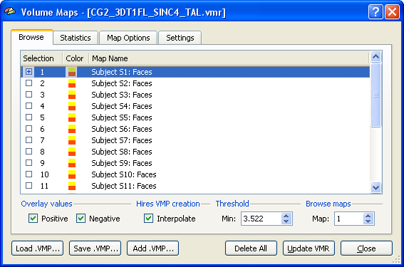
The group assignment and covariate scores will be the same for each voxel (ROI), while the dependent measures are different for different voxels (ROIs). A multi-subject VMP or SMP will provide the dependent measurements for all subjects while the group assignment and covariate scores must be added in a second step to complete the design. In the following example, a multi-subject VMP is used as input, which is derived from a separate subject GLM. Section Creating Multi-Subject t and Beta/Contrast Maps describes how t values or beta values can be extracted from a multi-subject GLM for each subject, thus, allowing ANCOVA analysis also for standard fMRI experiments. The example uses simulated data with a strong correlation of a single covariate with the dependent variable in order to clarify what can be expected from adding a covariate in the ideal case. The snapshot below shows the multi-subject VMP within the Volume Maps dialog. The map list shows several sub-maps. Each row in the list corresponds to the dependent measure of one subject. In order that the ANCOVA dialog accepts such a multi-subject VMP, the names of the sub-maps must follow the convention "<Subject ID String>: <Dependent Variable String>". While the exact way how subjects are named does not matter, the strings for different subjects must be kept separate. The colon (":") is necessary to separate the subject name from the subsequent name of the dependent variable, which is "Faces" in the example. If each subject would have more than one condition, the names should look similar as: "S1: Cond1", "S1: Cond2", "S2: Cond1, S2: Cond2" and so on. Since the single-factor ANCOVA accepts only one dependent measurement per subject, we need exactly one entry per subject with the same name for the dependent variable ("Faces" in the example). In case of a fractional anisotropy group analysis, the name of the dependent variable could be called "FA" instead of "Faces". Section Creating Multi-Subject t and Beta/Contrast Maps describes how the names below are created automatically when extracted from a multi-subject GLM. For other cases (e.g. FA or cortical thickness maps), the multi-subject VMP or SMP can be built by adding maps obtained for the same measurement from individual subjects to the multi-subject VMP/SMP. The proper names can be entered after double clicking on the line of a sub-map.
Specifying the Design
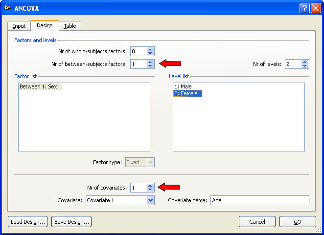
After specifying a multi-subject VMP (or SMP) as input in the Input tab, the ANCOVA dialog switches to the Design tab and sets automatically the design to a one between-factors model as indicated by value "1" in the Nr of between-subjects factors field. To extend this single-factor ANOVA model to a single-factor ANCOVA model, one or more covariates have to be added. In order to include one covariate, change the value to "1" in the Nr of covariates field. In the snapshot below, the name of the between-factor has been changed to "Sex" and the two levels (groups) of this factor have been changed to "Male" and "Female", respectively. You may want to save the created design for later use (e.g. ROI analysis) by using the Save Design button.
After specifying the design, the values of the covariate for each subject have to be entered as well as the assignment of each subject to group 1 ("Male") or group 2 ("Female"). This information is specified in the Table tab (see snapshot below).
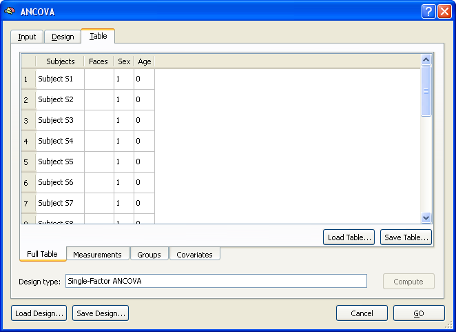
The Full Table tab of the Table tab shows an overview of the design. The left column shows the subjects in the same order and with the same names as read from the multi-subject VMP / SMP. The second column shows the dependent variable ("Faces"). Note that this column is empty since the values are different for each voxel of the map data. This column will be filled in case of a ROI analysis (see below). The third column shows the independent categorical variable "Sex" and the fourth column shows the covariate "Age". The latter two columns have to be filled with the correct values in order to complete the specification of the ANCOVA model. While these values can be entered in the overall table directly, it is helpful to switch to the respective sub-tables. The snapshot below shows the display after switching to the Groups tab.
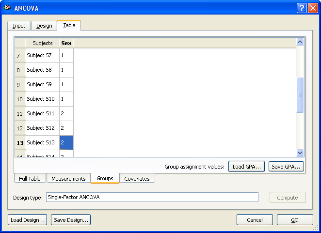
The values in this tab are auto-filled by simply assigning the first half of subjects to group 1 and the second half of subjects to group 2. In case of more groups, the values would be distributed in a similar way by dividing the number of subjects by the number of groups. If the subjects are ordered in the multi-subject VMP / SMP file accordingly, no change is necessary. Otherwise the correct assignment must be specified for each subject by simply entering the correct group ID (1, 2) in the respective field. You may also save a specific group assignment using the Save GPA button (GPA = group assignment). The Load GPA button can be used later to re-establish a specific assignment. This is useful in case you have multiple data sets with the same order of subjects.
The last step would be the same for any design with one between-subjects factor. In case of an ANCOVA model, the final information to be provided are the subject-specific scores of the covariate. These can be entered in the Covariates tab as shown in the snapshot below.
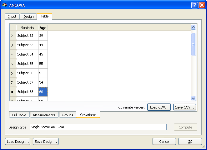
The covariate values can be entered for each subject by simply typing the correct value in the cell of the respective subject. The values can be also loaded from disk if the covariate values had been saved before (or entered in a file outside of BrainVoyager) using the Load COV and Save COV buttons.
This completes the specification of the ANCOVA model for the used example data set. The specified ANCOVA can be calculated for the data of each voxel by clicking the GO button resulting in a .AVA file with the resulting data.
Inspecting ANCOVA Map Results
To inspect the results of the ANCOVA calculation and to ask specific questions, the Overlay RFX ANCOVA Tests dialog must be invoked from the Analysis menu and a desired AVA file must be loaded using the Load .AVA button. If a ANCOVA AVA map has just been calculated the overall F test will be shown on the VMR data and the AVA data residing in working memory will be used (no loading necessary). The snapshot below shows the result of the overall F test highlighting a region with different mean effects for the two groups "Male" and "Female". It would be interesting to know whether the covariate helped to get the clear result, which could be done by running the same model without the covariate (see below). Since the covariate will help in case that it is linearly correlated with the dependent variable, another way to show whether the covariate is "effective" is to show a corresponding correlation map. This can be done by clicking the Covariate correlation option or the F test: r > 0 option. The first option will provide a map with the respective correlation value at each voxel whle the latter will produce an F map. In our example data, the covariate shows indeed high correlation values for the voxels in the region detected with the overall F test.
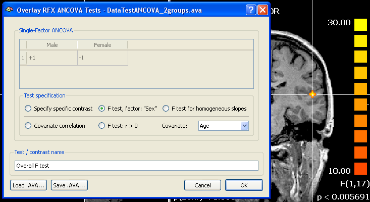
It is also possible to compare specific groups using the Specify specific contrast option. Since in the example data there are only two groups, the comparison would not lead to a different result, except that a t map would be calculated and the two-tailed test would indicate which group has a greater mean at each voxel (red vs blue colored voxels). Such a contrast would be done as usual by giving one group a "+1" value and the other group a "-1" value in the contrast table (see snapshot above). As a prerequisite of the ANCOVA, the correlation of the covariate with the dependent variable should not differ across groups. This assumption can be tested with the F test for homogeneous slopes option. The resulting map should not lead to significant F values in the regions detected with the overall F test. If areas of interest show significant F values after this test, a standard ANOVA model should be used (at least for interpretation of those regions), i.e. dropping the covariate. More insights in the effects of the covariate and whether prerequisites are met are provided in the numerical and graphical output provided by the ROI ANCOVA analysis.
ROI ANCOVA Analysis
ANCOVA models can not only be applied to (multi-voxel) map data but also to data sets from a single data source, which is typically a region-of-interest (ROI) in the context of neuroimaging data. While the dependent measures can be manually entered, they can be also loaded from specific file types (".ATD" and ".DPV"). Both the VOI Analysis Options and the Patch-Of-Interest Analysis Options dialog contain routines to save data from multi-subject GLMs / VMPs and SMPs in ".ATD" ("ATD = ANCOVA table data) format, which can be read directly into the ANCOVA dialog.
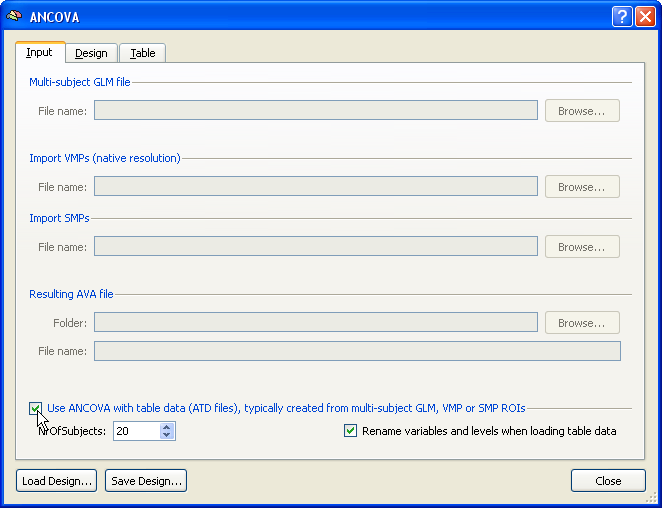
To start a single data source ANCOVA analysis, the Use ANCOVA with table data option has to be checked in the Input tab of the ANCOVA dialog. While the number of subjects might be determined directly from a .ATD file, it is recommended to also specify the number of subjects to analyze in the Number of subjects field.
The design can be specified in the same way as described above using the fields in the Design tab. If a .ATD file is available, you may also load this file directly, which will set the design including names for the dependent variable and factors (but not for levels of a factor). An example .ATD file might look like this:
FileVersion:          2

NrOfSubjectRows:      20
NrOfDataColumns:      1
NrOfGroupingColumns:  1
NrOfCovariateColumns: 0

"Subjects"       "Faces "  "Sex"
"Subject 1"       2.89437    1
"Subject 2"       5.25764    1
"Subject 3"       6.93016    1
  :
In this example, the grouping factor is already included but not the covariate. The ".DPV" file format does not attempt to read the data for a full design, but only contains values for the dependent variable (DPV = dependent variable). A typical .DPV file looks like this:
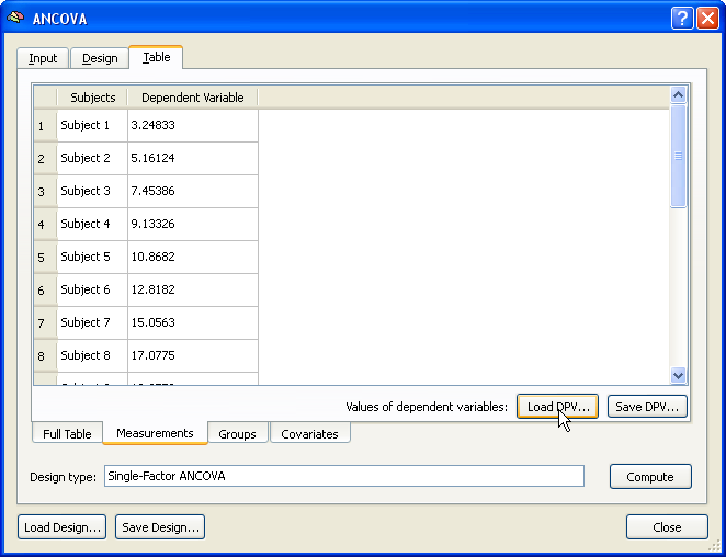
NrOfSubjectRows: 20
NrOfDataColumns: 1
 3.24833
 5.16124
 7.45386
 :
After specifying the design as described in the "Specify the Design" section, the .DPV file shown above has been loaded by using the Load DPV button in the Measurements tab of the Table tab. Note that the values per subject could also be entered manually. The group assignment can be done next as described above for the multi-subject VMP case.
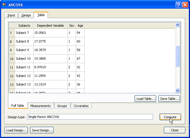
Finally, the covariate values are entered using the Covariates tab. If the values have been saved in the multi-subject VMP step (see above), e.g. as "Age.cov", the subject-specific scores can be incorporated in the ANCOVA model simply by loading this file from disk using the Load .COV button in the Covariates tab. The snapshot below shows the obtained result after entering all the data for running the ANCOVA model. This overview display is obtained by switching to the Full Table tab. The ANCOVA calculations for the provided data are performed after clicking the Compute button at the right lower section of the Table tab.
The result of the ANCOVA calculation is displayed numerically in several tables and a summary plot. The output starts with a section showing the name and the levels of the between-subjects (grouping) factor (factor "Sex" with levels "Male" and "Female" in the example data).
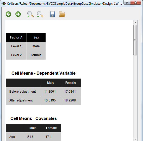
The next table shows the mean values for each group. The original mean values are shown in the “Before adjustment†row. The "After adjustment" row shows mean values corrected for different mean values of the covariate in the diferent groups: If one group (despite randomization) contains a different mean of the group's covariate scores, the mean value of the dependent variable will be increased/decreased for that group as compared to the other group in case that the covariate is positively/negatively correlated with the dependent variable. The adjusted means, thus, compensate for different starting values with respect to the covariate scores. The mean values of the covariate is shown in the next section for each group.
The next section of the output (see snapshot below) shows the main table indicating how much variance is explained by the between-subjects factor ("Treatments" row) and whether the means are significantly different from each other (F and p values). For the example data the significance of the "Sex" factor is highly significant. When running the model without the covariate, the factor will not reach significant indicating the important role of the covariate (high correlation with the dependent variable) in the example data. A more detailed description of a direct ANOVA - ANCOVA comparison can be found in the blog entry The 'C in ANCOVA.
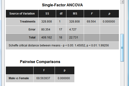
The next section (see snapshot above) shows statistical results for all pairwise comparisons. Since the example data contains two groups, only one comparison ("Male vs Female") is presented with the same F value as for the overall F test. The next table (see snapshot below) shows the correlation value of the covariate ("Age") with the dependent variable, which is extremely high (r = 0.93) for the example data. The F and p values indicate that the correlation value is different from zero with very high significance.
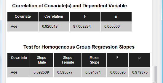
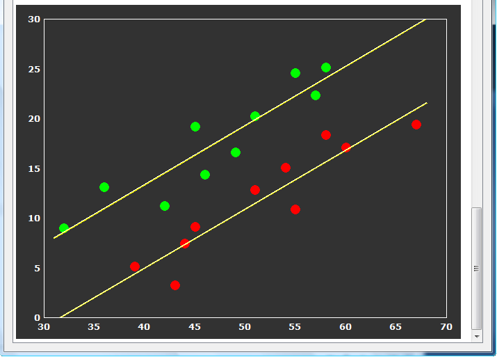
The last table tests whether the correlation of the covariate with the dependent variable does not significantly differ across the levels (groups) of the independent (grouping) factor. In the example data the F test for homogeneous group regression slopes is not significant allowing to interpret the obtained statistical results. In case that this test is significant (i.e. p < 0.05), the ANCOVA model should not be interpreted and replaced by a corresponding ANOVA model without the covariate. The slopes for each group are also plotted in the final output of the ANCOVA showing a scatter plot of the data points with the covariate on the x axis and the dependent variable on the y axis (see snapshot below). This graph also indicate that the variability in the groups around the regression slopes is much reduced as compared to the variability around the mean (not shown). For further details, check the blog entry The 'C' in ANCOVA.
Copyright © 2023 Rainer Goebel. All rights reserved.