BrainVoyager v23.0
Population Receptive Field Estimation
Introduction
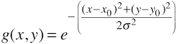
Early visual areas have been mapped and delineated since the early years of fMRI using retinotopic mapping experiments that use ring and wedge stimuli to create visual field maps (Sereno et al., 1995). More recently, an alternative technique has been proposed that uses a model-driven approach to estimate neuronal population receptive fields (pRFs) as the basis to create visual field maps (Dumoulin & Wandell, 2008). The pRF approach estimates a model of the population receptive field for voxels in visual cortex that best explains measured fMRI responses resulting from a series of various visual stimuli. The visual stimuli may be the same as used in conventional retinotopic experiments (rings and wedges) but also other stimuli can be used (e.g. bars at different positions and orientation). The pRF method is, however, not only an alternative method to map early visual areas since the model-based approach is able to estimate additional neuronal quantities such as estimation of the population receptive field size. The standard model (Dumoulin & Wandell, 2008) that is usually estimated from fMRI data is specified as a Guassian model with 3 free parameters, the position, x0 and y0 of the population receptive field as well as its standard deviation (i.e. its size) σ:
A time course can be generated from such a model by sampling the visual stimuli within the receptive field during an experiment: the position and size of a model will then generate a model time course that will exhibit positive responses each time when a stimulus falls within its recpetive field. Note that a receptive field located at another location will produce a different time course since the stimuli will usually fall in the other model's receptive field at different moments in time. Further note that a model with a larger receptive field size will be influenced by stimuli that are further away from the pRF center than an alternative model with a smaller receptive field size even if the center of the two models is located at the same position in the visual field. if "rich" visual stimuli are used, each model will, thus, produce a unique predicted time course. The predicted time courses from different pRF models can be compared with the measured time course of a specific voxel (or vertex) and the model will be selected for that voxel if its associated time course best explains the observed time course. More specifically, a generated model time course serves as a predictor in a GLM (instead of protocol-derived predictors) and the amount of explained variance is recorded. Instead of one set of protocol-derived predictors, many GLMs will be performed for a single voxel each with a different model time course as predictor in order to find the model that leads to the highest explained variance of the voxel's time course. In order to allow a proper comparison of a model time course with observed fMRI data, a generated model time course needs to be convolved with a (standard) hemodynamic impulse response function.
Note that the pRF approach is not limited to the (standard) Gaussian model, i.e. other models can be employed that may estimate, for example, non-circular receptive fields or that form a "mexican hat" shaped receptive field with a negative region surrounding a positive interior region. Several aspects of performing good pRF fMRI studies are evaluated by Senden et al. (2014). Furthermore, the pRF approach is not limited to retinotopic mapping and can be used to estimate different neuronal population quantities such as sound frequencies in auditory cortex. It is also expected that sub-millimeter features measured with ultra high-field fMRI (e.g. Yacoub et al., 2008; Zimmermann et al., 2011) will be modeled by the pRF approach in the future. Generally speaking, the pRF method is attractive for basic and applied neuroscience since it quantitatively couples fMRI signals with receptive field properties of (visual) neurons measured at the micron scale.
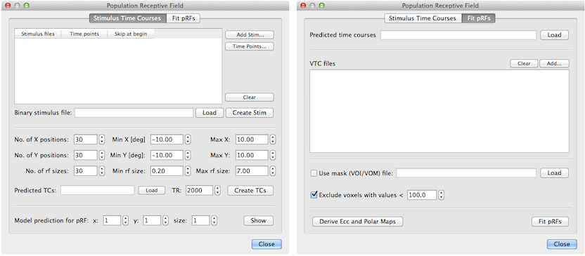
The basic pRF method has been implemented in BrainVoyager (starting with version 2.8) and it is accessible through the Population Receptive Field dialog (see above) that can be invoked using the Population Receptive Field Estimation item in the Analysis menu. The dialog contains two tabs; the first one, Stimulus Time Courses, uses provided stimulus data to calculate predicted model time courses while the second tab, Fit pRFs, is used to perform the actual model fitting. The implemented multi-threaded pRF model fitting procedure operates both for voxels of VMR-VTC projects as well as for vertices of SRF-MTC data.
References
Dumoulin, S.O., Wandell, B.A. (2008). Population receptive field estimates in human visual cortex, Neuroimage, 39, 647-660.
Sereno, M.I., Dale, A.M., Reppas, J.B., Kwong, K.K., Belliveau, J.W., Brady, T.J., Rosen, B.R., Tootell, R.B. (1995). Borders of multiple visual areas in humans revealed by functional magnetic resonance imaging. Science, 268, 889-893.
Senden M, Reithler J, Gijsen S, Goebel R (2014). Evaluating population receptive field estimation frameworks in terms of robustness and reproducibility. PLoS One, 9, e114054.
Yacoub., E., Harel, N., Ugurbil, K. (2008). High-field fMRI unveils orientation columns in humans. PNAS, 105, 10607-10612.
Zimmermann, J., Goebel, R., De Martino, F., van de Moortele, P.F., Feinberg, D., Adriany, G., Chaimov, D., Shmuel, A., Ugurbil, K. & Yacoub, E. (2011). Mapping the organization of axis of motion selective features in human area MT using high-field fMRI. PLoS One, 6, e28716.
Copyright © 2023 Rainer Goebel. All rights reserved.