BrainVoyager v23.0
ADC, FA and Color Direction Maps
Diffusion maps (as well as tensor visualization and fiber tracking) can be performed if a subject's DDT file has been linked to a loaded VMR file. For proper calculations it is important that a right DDT file is used, which has been calculated from VDW data residing in the same space as the current VMR data set.
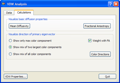
As described earlier, the DDT file contains, for each voxel, three estimated eigenvectors and associated eigenvalues, which can be used to calculate various diffusion maps (see below). To calculate and visualize these maps, invoke the VDW Analysis dialog from the DTI menu and switch to the Calculations tab. If a DDT file has been linked, the Mean Diffusivity, Fractional Anisotropy and Color Directions buttons will be enabled and the calculation of the respective maps will be possible. If these buttons are disabled, you need to link a DDT file first.
Mean Diffusivity Maps
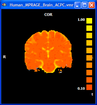
In a mean diffusivity or ADC (apparent diffusion coefficient) map, all three eigenvalues of a voxel's tensor are simply averaged (or summed) to quantify the amount of diffusion. The snapshot below shows some slices of a DTI data set with a mean diffusivity map, which can be obtained by clicking the Mean Diffusivity button in the Visualize basic diffusion properties field. The snapshot depicts a coronal slice of a calculated Mean Diffusivity VMP showing that diffusion is highest in cerebro-spinal fluid (ventricles and large vessels) indicated by yellow color shades and weaker in white and grey matter indicated by orange colors.
Fractional Anisotropy Maps
If all three eigenvectors of a voxel have an eigenvalue of similar magnitude, the diffusion is isotropic and the shape of the diffusion tensor will be close to a sphere. If the eigenvalue of one eigenvector is large and the other two eigenvalues are small, diffusion is highly anisotropic and the shape of the diffusion tensor will look like a cigar. The most common measure quantifying anisotropy is fractional anisotropy (FA) determining the fraction of the diffusion tensor, which can be ascribed to anisotropic diffusion. FA is calculated as the normalized variance of the three eigenvalues:
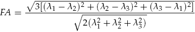
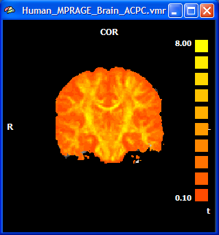
The FA value varies between 0 (isotropic diffusion, shape of a sphere) and 1 (infinite anisotropy, shape of a line). The snapshot below depicts the same coronal slice as above with a superimposed FA map (VMP) obtained after clicking the Fractional Anisotropy button in the Visualize basic diffusion properties field. The figure shows that anisotropy is high (yellow color) in white matter but low (orange color) in grey matter.
Color Direction Maps
While FA maps reveal differences in anisotropy across space, they do not reflect any direction information. Color Direction maps are able to visualize direction information about diffusion by color-coding direction information from the eigenvectors. In the most common approach, the x, y and z components of the eigenvector with the largest eigenvalue are used for color coding. The color red, for example, can be used to indicate diffusion along the left/right axis (eigenvector [1, 0, 0] ), green for diffusion along the anterior/posterior axis (eigenvector [0, 1, 0] ) and blue for diffusion along the inferior/superior axis (eigenvector [0, 0, 1] ). Diffusion along intermediate directions can be visualized by appropriately mixing of the three basic colors. Note that although an eigenvector points in a specific direction, the measured diffusion occurs both along the direction of the eigenvector as well as in the opposing direction. An eigenvector thus must be interpreted as indicating an axis of diffusion. The snapshot below shows the same coronal slice as above with different versions of color direction maps obtained by clicking the Color Directions button in the Visualize direction of primary eigenvector field.
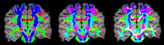
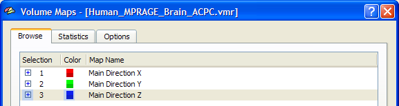
The difference of the three images is that different color mixing modes are used. In the image on the left the Show only max color component option has been checked prior to clicking the Color Directions button. With this option in effect, only the cmponent with the maximum value is shown in the respective color. While this does not reflect information about oblique directions, the resulting visualization may be easier to comprehend than one of the other visualizations. The image in the middle has been obtained using the Show mix of two largest color components option (default). This option reveals also information about oblique directions considering the two largest direction components for color coding. The image on the right has been obtained using the Show mix of all color components option. This option reveals the full information about the direction of a voxel's diffusion axis considering all components for color coding. While the FA and Mean Diffusivity maps are stored as single volume maps, the color direction maps are stored as a set of three volume maps, each coding one component (x, y, z) of the maximum eigenvector. The snapshot below shows the (native resolution) Volume Maps dialog with the three color maps. Parameters of these maps, including the colors used and the thresholds can be changed as wilth any other (statistical) volume map.
The color direction maps shown above are mainly confined to white matter voxels. Besides having used a brain mask file when estimating the tensors, this is mainly the result of using the Weight with FA option in the Visualize direction of primary eigenvector field, which uses the magnitude of the FA value at a voxel to blend the color information with the background (anatomical) intensity information.
Copyright © 2023 Rainer Goebel. All rights reserved.