BrainVoyager v23.0
Decoding pRF Models
After estimating pRF models in volume and surface space, the resulting maps can be used to visualize estimated parameters (location, pRF size) in visual cortex as well as useful derived maps such as eccentricity and polar angle maps. The polar angle map is particularly useful to delineate early visual areas revealing the mirror-symmetric layout of visual areas V1, V2 and V3 that meet at explicitly represented horizontal and vertical half-meridians.
An additional application of pRF maps is to visualize the location and size of the estimated receptive field of voxels (and vertices) in visual input space, i.e. the information represented by a voxel is projected (decoded) into the visual field. BrainVoyager offers two ways to decode pRF models. The first approach simply visualizes the model parameters of a specific voxel or vertex at the corresponding location in visual space. The second approach performs this "back-projection" for many voxels taking into account the activation level of a voxel, i.e. the visualization "strength" of the pRF in visual input space is weighted by the activation level of a voxel; when integrating this information from a distributed activation pattern in (sub-parts of) early visual cortex, it should be possible to reconstruct the visual stimulus seen (or imagined) by the participant.
Visualizing pRF models of selected positions in the visual field
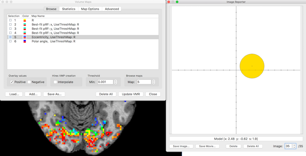
When a pRF volume or surface map has been created or loaded, pRF models are automatically shown in visual input space when CTRL-clicking (CMD-clicking on Mac) a voxel or vertex. The figure above shows a loaded pRF volume map; after clicking a voxel (see black mouse pointer in screenshot above), the pRF model parameters (x, y, sigma) are retrieved from the voxel's map values and displayed at the respective position and size in the visual field (see visualization on right side of screenshot above). The created visualization is added to Image Reporter and the parameters of the pRF model are shown in the text field below the created image. If Image Reporter is not currently visible, it is shown automatically. Clicking on another voxel will create a new pRF visualization in input space that will be again added to Image Reporter; this allows to run through all created pRF visual field visualizations by using the Image spin box of Image Reporter. The selected pRF model is visualized as a disk with a radius corresponding ot the receptive field size (parameter 3, sub-map 4). In case that an eccentricity map is available, the color of the disk reflects the eccentricity (distance from center) of the code; this color-code is also shown in case that another sub-map (e.g. "Polar angle" sub-map) is currently visualized. Note that the stimulus reconstruction method (see below) projects a gradual visualization of the pRF Gaussian shape in the visual field.
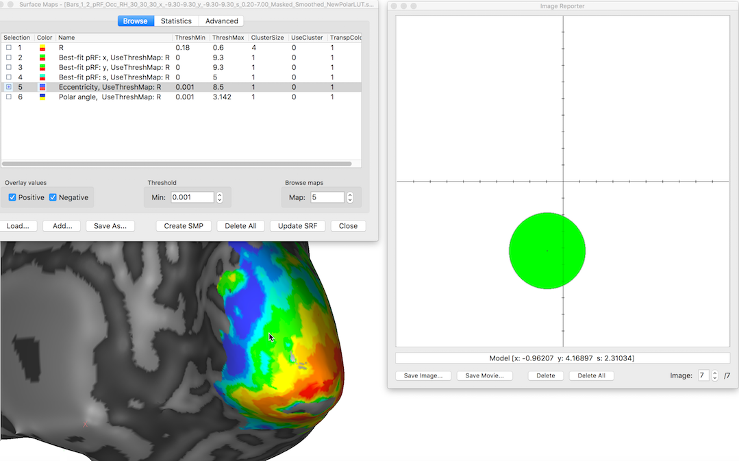
The screenshot below shows the same procedure after loading a pRF surface map visualized on a (inflated) cortex mesh. After a vertex is CTRL-clicked (CMD-clicked on Mac), the pRF model parameters of the selected vertex are retrieved from the respective surface sub-mpas (2, 3, 4) and converted in a display of the pRF in visual input space that is added and shown in Image Reporter. BrainVoyager provides this functionality only if it detects a pRF map checking that the names of the sub-maps 2, 3 and 4 contain the sub-string "pRF". In case that one generates pRF maps using custom programs, one should make sure that the produced map names follow this heuristic in order to get this pRF visualization functionality. In order to get eccentricity-based color-coded pRF disks, an eccentricity sub-map (position 5) needs to be available and the sub-map name must contain the sub-string "Eccentricity".
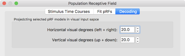
As default, the pRF input space visualization uses an extend of 10 degrees of visual angle to the left, right, above and below from the center, i.e. 20 degrees in total in horizontal and vertical direction. The center (x=0 degrees, y = 0 degrees) and the degrees of visual angle are visualized in the image with a respective horizontal and vertical line crossing in the center and depicting tick marks indicating visual angle along the axes (... -2, -1, +1, +2...). The extent of visual space can be adjusted using the Visualization tab of the Population Receptive Field dialog (see screenshot below). Change the values in the Horizontal visual degrees and Vertical visual degrees spin boxes to adjust the displayed visual space; note that it is recommended to use the same value for both dimensions even if one dimension covers a larget visual space. The values entered in this dialog are used immediately (after closing the dialog) and they are stored as permanent settings to disk, i.e. the entered values persist across BrainVoyager sessions (until they are changed again).
Visual Stimulus Reconstruction from Distributed Activity Patterns in Visual Cortex
For the stimulus reconstruction approach, a distributed activity pattern is converted into an image in the visual field by projecting the pRF models of active voxels or vertices into a visual field representation; the projection strength ("brightness") of a pRF Gaussian shape model at a particular location in the visual field depends on the activity amplitude of the voxels (or vertices). This procedure in effect "decodes" an activity pattern in visual cortex in a visual field representation reconstructing a visual image of a stimulus. Note that the decoding is not limited to activity patterns from stimuli during pRF estimation but can be applied to any activation pattern resulting e.g. from new input stimuli or from internally generated mental images as long as early visual cortex is activated in a topographically meaningful way.
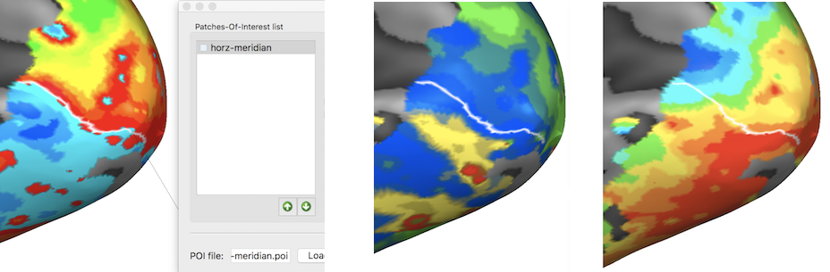
The reconstruction procedure can be demonstrated by selecting vertices along the calcarine sulcus, which should decode the pRF models at these voxels into a horizontal meridian visual image. The screenshot above (left side) shows how vertices along the upper, lower border of the visual field representation have been selected in the right hemisphere of an example data set using the estimated pRF map for parameter "y" (map 2 in a standard pRF map). The snapshots on the right show that finding the horizontal meridian is more difficult on a conventional polar angle map (second image) and not detectable on a eccentricity map (third image). The marked vertices have been converted in a POI called "horz-meridian" containing the vertices along the path using the Define Patch-Of-Interest (POI) item in the local context menu of the surface window.
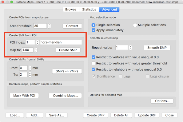
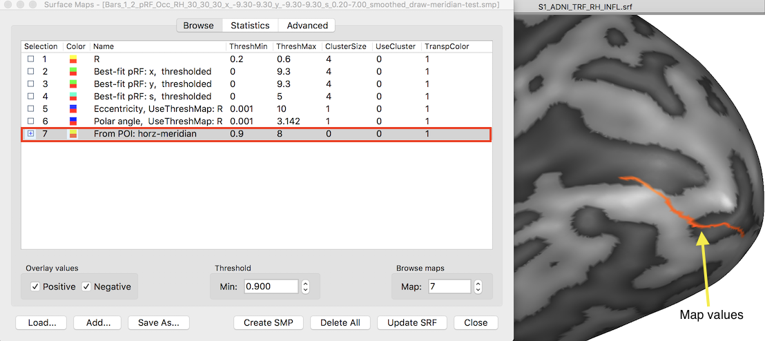
In order to use the pRF reconstruction tool, at least one sub-SMP is required as input, usually from measured responses to stimuli (a POI can not be used directly). For demonstrating the reconstruction process, the POI vertices will be used. Since BrainVoyager 20.4 it is possible to convert a patch-of-interest into a surface map using the Create SMP button in the Create SMP from POI field that is available in the Advanced tab of the Surface Maps dialog (see red rectangle in screenshot above). The POI index spin box can be used to select the desired POI; the name of a selected POI will be shown in the neighboring POI name text field. The Map to spin box can be used to adjust the map value (default 1.0) that will be assigned to the vertices in the POI - all other vertices will receive value 0.0. The screenshot below shows the resulting sub-map (map 7 in the surface map list after clicking the Create SMP button on the left and the thresholded map values (threshold set to 0.9 as default) of the vertices from the source POI on the right. Note that the map has been added to the existing pRF maps, which is important for using the map as input for decoding; maps can be of course also added by using the Add button.
As a side note (not show here), similar "drawing-based decoding" can also be done using pRF volume maps by creating a VMP sub-map from VOIs that are converted from drawn voxels in the VMR using the Define VOI procedure; the VOIs can then be converted to VOMs using the Create VOMs dialog, which finally can be converted to VMPs using the Create VMP button in the Visualize VOMs dialog. When no map values are attached to the VOM (only ROI coordinates in the resolution of maps), the values of the respective voxels in the created sub-map will be set to 1.0
Activity maps can be reconstructed using the tools in the Visual input reconstruction field of the Dcoding tab in the Population Receptive Field dialog (see screenshot below). The pRF plus activity maps text field will show the currently created or loaded SMP file. If no SMP is currently available, a pRF SMP can be loaded using the Load button next to the pRF plus activity maps text field. Note that a standard pRF map contains 6 sub-maps and at least one activity map needs to have been added. The Activity maps from and Activity maps to spin boxes contain the range of activity maps that will be decoded. As default one activity map (no. 7) is set as the decoding target. Optionally, a mask file (VOM/VOI in volume space, POI in cortex surface space) can be loaded using the Load button next to the Mask file text field. This can be used to restrict the activity pattern to sub-regions of visual cortex, e.g. to separate reconstruction from V1, V2 and V3 from each other vs reconstruction from all areas together. The decoding process is performed for the specified sub-map(s) by clicking the Reconstruct button.
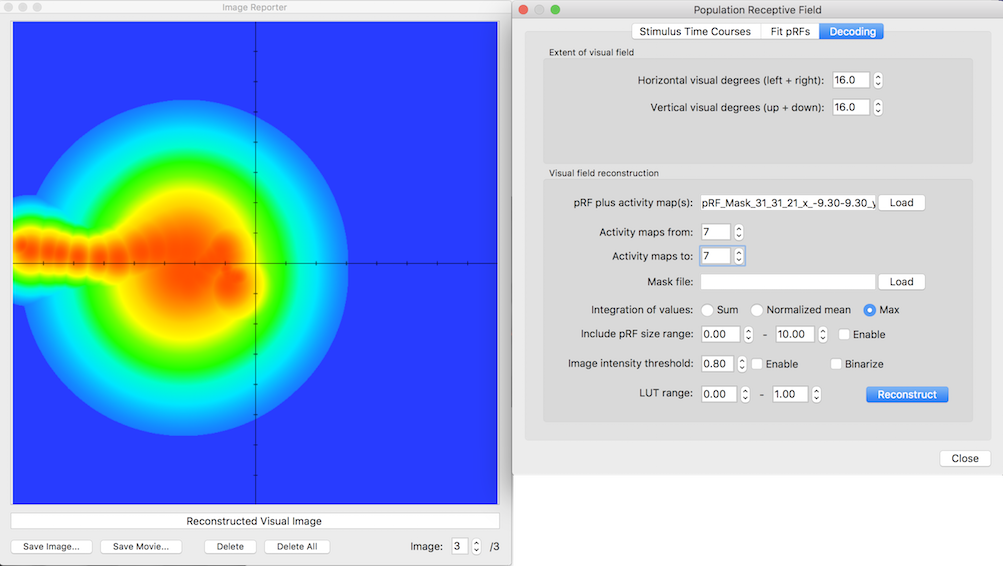
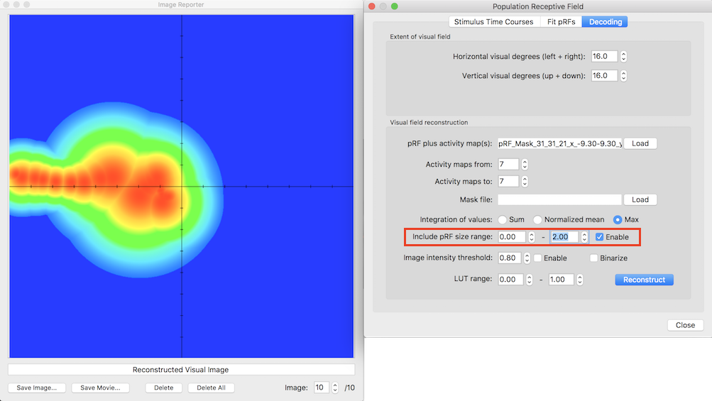
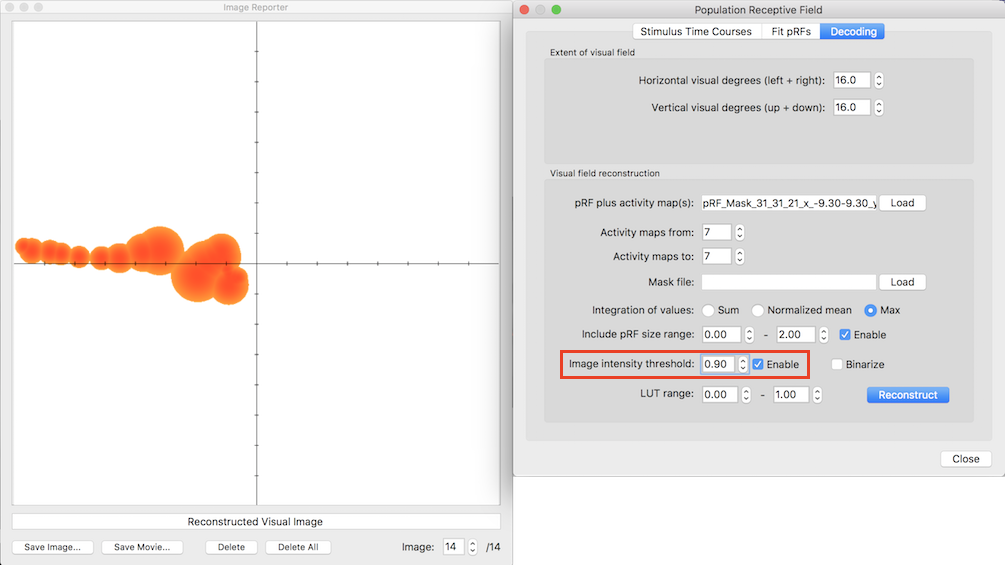
The left side of the screenshot above shows the reconstructed visual representation of the horizontal meridian map as an image in Image Reporter. As expected, the activity is confined around the left half meridian. Around 2 - 4 degrees eccentricity there are some larger receptive field sizes that "blurs" the reconstructed image. There are two possibilities to filter the reconstruction process. First, the Include pRF size range spin boxes can be used to restrict the used pRF models to those with a pRF size parameter in the specified range. As default this filter is turned off and can be turned on by checking the Enable option on the right side of the range spin boxes. Even if turned on the default range is rather large (pRF size (sigma) prarameter: 0.0 - 10.0). The screenshot below shows the result after clicking the Reconstruct button again when setting the pRF size to a range of 0.0 - 2.0 (see fields in red rectangle on right side).
After the pRF size restriction, the reconstructed image follows the horizontal left half-meridian even closer. Another filter can be applied to threshold the intensity values of the reconstructed image. The intensity values are scaled from 0.0 to 1.0 according to the smallest and largest reconstructed value in the reconstructed image; the 0.0-1.0 intensity range is mapped to a standard blue, green, yellow, red color range. The intensity range can be thresholded by turning on the Enable option on the right side of the Image intensity threshold spin box. The screenshot below shows the result after clicking the Reconstruct button again when using a threshold of 0.8 (see fields in red rectangle on right side).
In case an image is thresholded, the result can be also binarized, i.e. the pixels with a value above the threshold will be shown in one color (black) while the sub-threshold pixels will be shown in another color (white background). The screenshot below shows the result after clicking the Reconstruct button when also the Binarize option has been turned on.
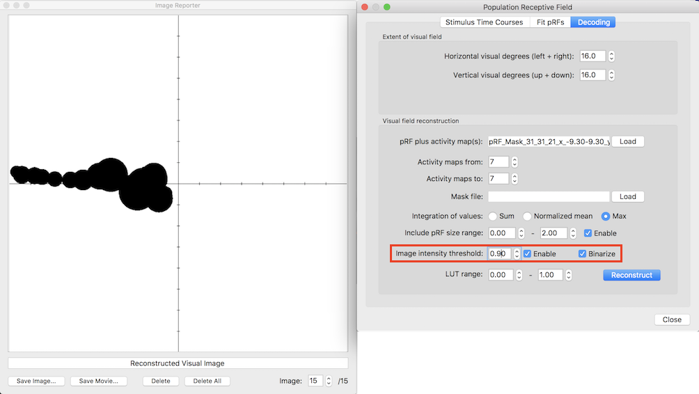
The reconstructed image now nicely reflects the horizontal half meridian. The provided options are also useful to optimize the visulization when decoding activity patterns emerging from fMRI measurements. In this application the maps added for visual field reconstruction result from analyzed (averaged or single-trial) responses to specific stimuli. The screenshot below shows four sub-maps added to the pRF maps in the Volume Maps dialog. These sub-maps contain activity patterns evoked by four presented letter shapes (H, T, S, C) that were recorded in an fMRI study performed in the same session as the pRF estimation (Emmerling et al., 2016). The map for the presented letter H is shown ovelaid on the VMR of the participant on the left side of the screenshot.
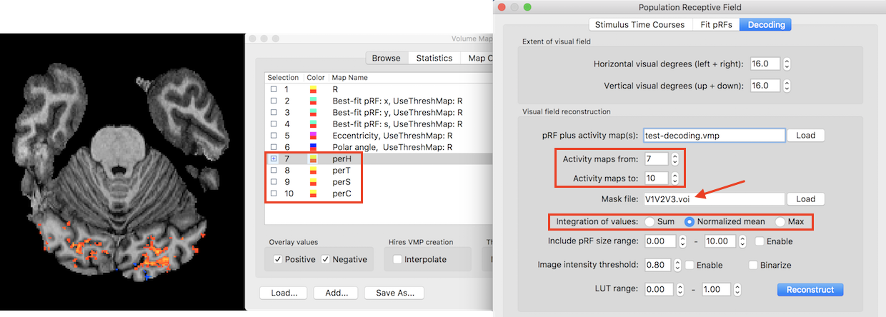
The right side shows the Decoding tab of the Population Receptive Field dialog. The Activity maps from and Activity maps to values have been adjusted to include the four perceived letter sub-maps (7 - 10). Furthermore, a VOI mask file has been loaded (V1V2V3) to limit the decoding process to voxels in early visual cortex. In separate runs, decoding can be performed for other ROIs, e.g. V1 or V2 or V3. Note that the intensity value of a pixel from one pRF projection is the product of a voxel's activation and the value of the Gaussian weights extending 2 standard deviations of the pRF size value around the projected location. The Integration of values field can be used to specify how multiple pRF projections are integrated at a pixel to determine the final intensity output value in the visual field image. The figure below shows the reconstruction of the four letters using the summation and normalized mean approach:
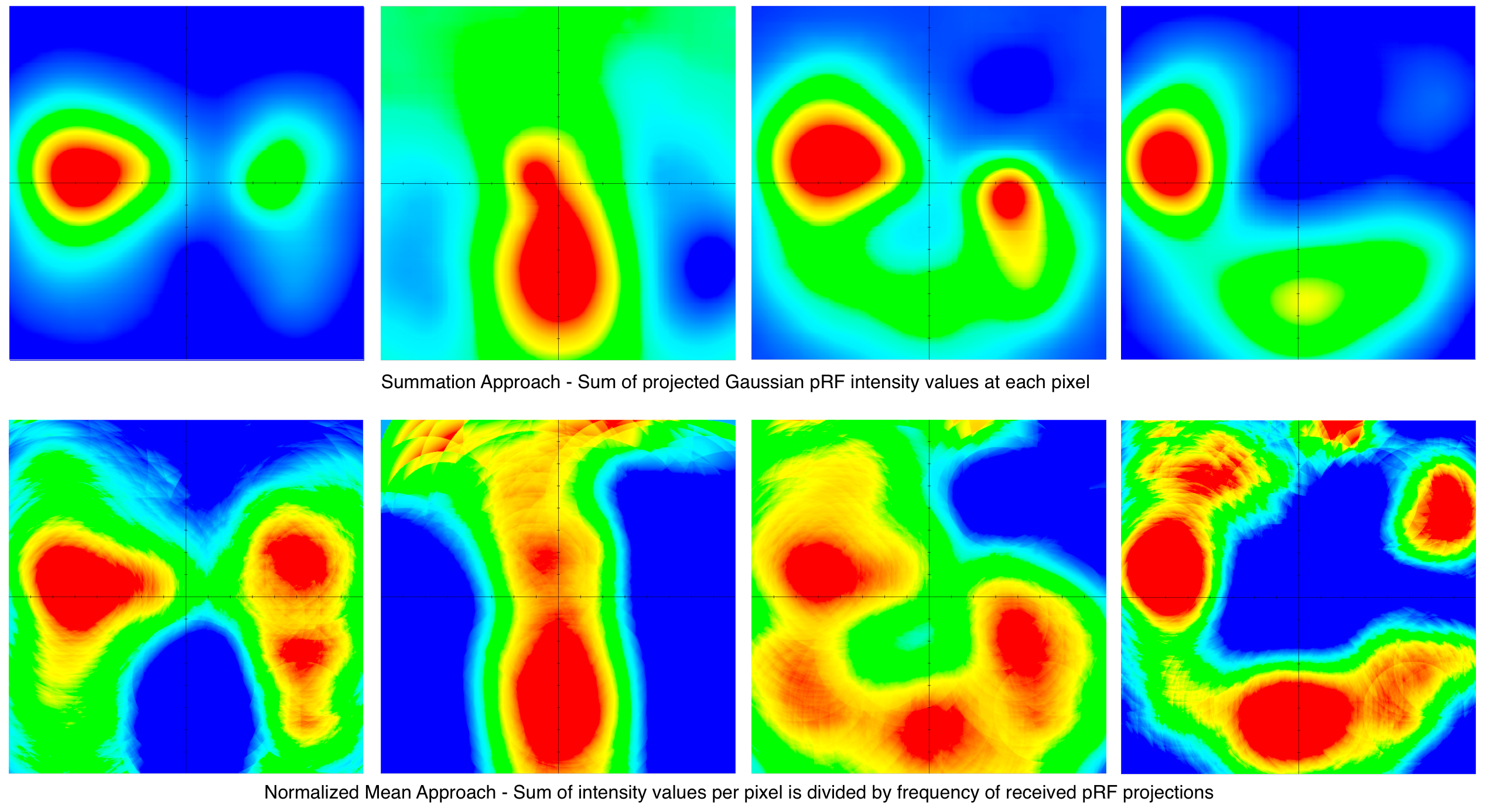
The columns 1-4 of the figure above show the reconstructed letters H, T, S and C. The first row has been reconstructed using the Sum option in the Visual field reconstruction section in the Decoding tab of the Population Receptive Field dialog; with this approach, projected values at each pixel are simply added up to result in a final intensity value. This reconstruction approach reveals that some areas in the visual field receive Gaussian pRF projections from many voxels (red areas) while other regions receive less projections. This can be compensated by using the Normalized mean option (default); in this approach a pixel's summed intensity value is divided by the amount of pRF projections that the pixel has received. The second row of the figure above indicates that this normalization approach leads to better approximations of the letter shapes presented to the participant during the fMRI scan. The Max option offers another approach (used in the horizontal meridian example abvoe) that records the maximal projected value at a pixel as its final intensity value.
Copyright © 2023 Rainer Goebel. All rights reserved.