BrainVoyager v23.0
Postprocessing of DNN Segmentation Results
When the DNN segmentation has finished tissue classification, BrainVoyager loads and shows the primary result as a stack of volume maps in the Volume Maps dialog (upper right dialog in screenshot below) containing for each voxel the probability estimates that it belongs to one of the 8 included tissue types. The corresponding VMP file is stored in the same folder of the input VMR / V16 files and the name will be recognized by the extension '[name]_tissue-probs-{slow | fast}.vmp' (see red arrow in screenshot below). The program provides meaningful names for the different tissue classes and overlays automatically the most important maps including White matter (map 2, red colors), Grey matter (map 3, green colors), CSF (map 4, blue colors) and Blood vessels (map 7, magenta colors). To turn on and off multiple maps, BV has enabled the Multiple selection option in the Advanced tab of the Volume Maps dialog.
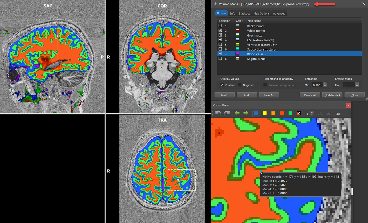
A useful way to inspect the tissue probabilities, especially across tissue borders, is to hover the mouse over respective regions, which will show the probability map values in the voxel info pane. Note that since BrainVoyager 22 this possibility is now also available in the Zoom View pane allowing to inspect tissue map values precisely for individual voxels. The lower right part of the screenshot above shows the mouse hovering over a voxel that has almost the same probabilities for both map 2 (white matter, p=0.497) and map 3 (grey matter, p=0.503). Since the grey matter probability is slightly higher than the white matter probability, grey matter wins in this case. Below it is shown how probabilities are transfromed into discrete non-overlapping tissue labels that will be stored as volumes-of-interest (VOIs).
Next to the Volume Maps dialog, also the DNN Segmentation Postprocessing dialog (see below) will be automatically opened after the DNN has finished calculating tissue probabilities. Note that you can open this dialog also anytime later using the DNN Segmentation Postprocessing item in the Volumes menu but to use its functionality a volume map with the DNN calculated tissue classification needs to be also loaded into the Volume Maps dialog.
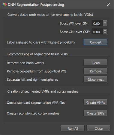
The dialog provides a series of buttons that launch several postprocessing steps starting with conversion of the probability maps into non-overlapping VOIs and ending with the creation of hemisphere volumes and cortex meshes. The first step is executed by clicking the Convert button, which converts the tissue probability maps into non-overlapping tissue segments. These non-overlapping segments are represented as VOIs in the appearing Volume-Of-Interest Analysis dialog (see lower left part in the screenshot below). The names of the VOIs are the same as used in the Volume Maps dialog but the Background entry has been dropped since the background is not modelled with a separate VOI. The conversion from probability maps to VOIs assigns a voxel to that VOI that has the highest probability value across tissues. Only if the 'Background' probability map 'wins', no VOI is assigned. The postprocessing dialog offers the option to 'boost' grey or white matter probabilities, which can be used to expand grey matter more towards CSF or white matter (or vice versa) if desired. If, for example, the Boost GM over CSF value is set to a postive value (e.g. 0.2), the chance for grey matter voxels to win transitional voxels at the GM / pial border will be increased. Note that boosting is only performed for voxels where the two involved tissue types have the two highest tissue probabilities. Note also that you can create VOIs repeatedly from probability maps with different boosting values by clicking the Convert button. While it is usually not recommended to use the boosting feature, it might be helpful in some cases.
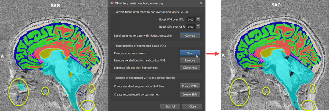
The next three steps offered by the DNN Segmentation Postprocessing dialog operate on the created tissue VOIs. Clicking the Clean button executes a simple 'cleaning' operation that removes small isolated pieces resulting in one (the largest) connected segment per tissue VOI (see some pieces highlighted with yellow ellipses in the screenshot below). Since BrainVoyager 22.0 this maximum component operation is also available in the Volume-Of-Interest Analysis dialog (Max Component button).
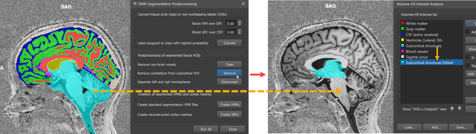
The next step is executed by clicking the Remove button. This step aims to detect and remove the cerebellum and other parts that are labelled in one large 'Subcortical structures' tissue segment. This step includes running MNI normalization (with a 1 mm rescaled version of the sub-millimeter data) to locate the mid-sagittal plane and (roughly) subcortical regions. If this step does not work satisfactorily, the later generated VMR volume segments can be further refined using standard editing tools. The 'remove cerebellum' operation results in a modified subcortical tissue VOI that is added to the list of VOIs with the name 'Subcortical structures Edited' (see orange arrows in screenshot below).
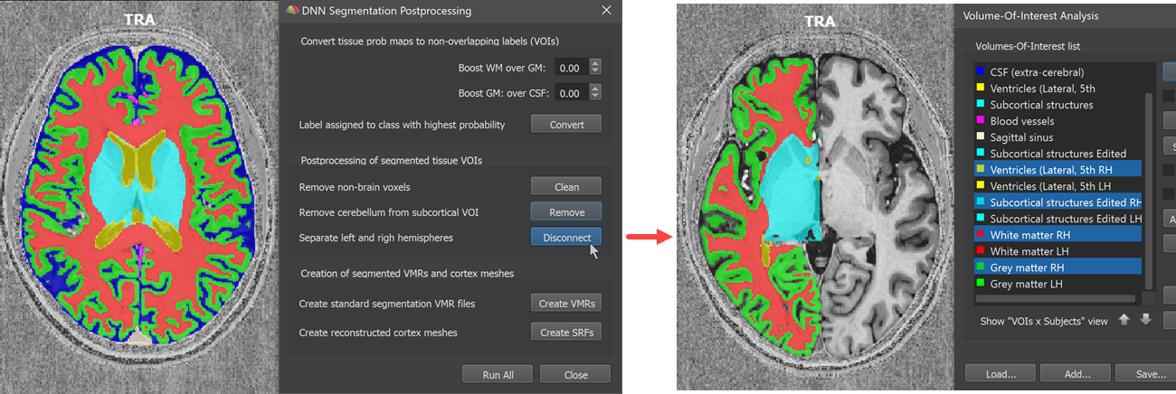
The next step is performed by clicking the Disconnect button. This step attempts to disconnect the tissue VOIs into a left and right hemisphere version. Like for the 'remove cerebellum' step, this step uses information from the MNI (backward) transformation calculated earlier. This 'disconnect' operation creates two new VOIs, a left ('LH') and right ('RH') from major tissue types. In the screenshot below the VOIs for the right hemisphere are visualized on an axial plane (shown on the left side in radiological convention).
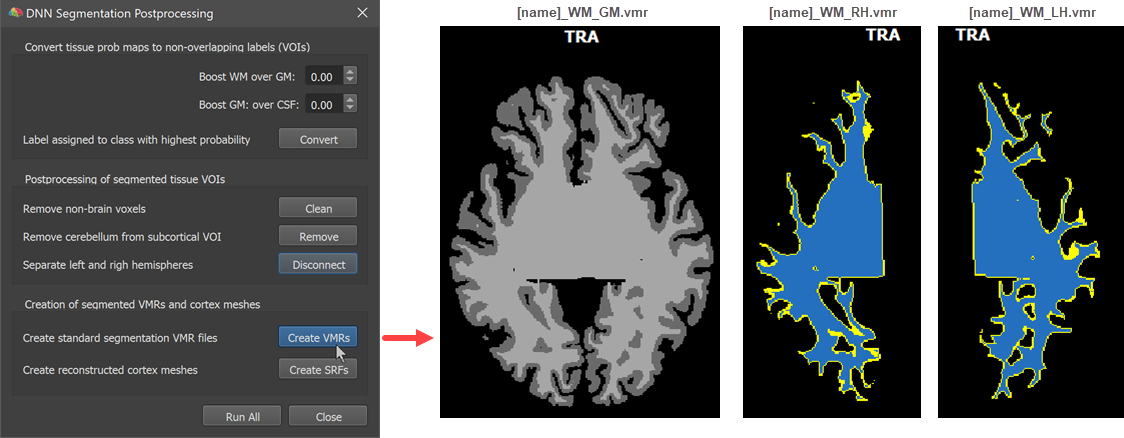
The final two steps expect successfully separated hemisphere VOIs that are used to create standard hemisphere volume segments as well as derived cortex meshes. After clicking the Create VMRs button (see screenshot below), the same volumes are produced as at the end of the advanced segmentation pipeline, including a standard 'WM-GM' volume with white matter (value 150) and grey matter (value 100) segmentations that can be used for cortical thickness analyses and laminar/columnar fMRI analyses. It also creates high-resolution left and right segmented ('blue') hemisphere volumes that can be further improved by manual editing if needed. It is also advised to run the standard bridge removal step before using the meshes for cortex-based alignment.
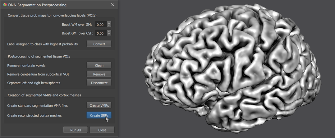
While meshes can be created from the generated volumes using standard tools, the program creates reconstructed and smoothed cortex meshes from the '[name]_WM_LH.vmr' and '[name]_WM_RH.vmr' segmented hemispheres and stores the resulting files ('[name]_WM_{LH | RH}_RECO.srf' and '[name_]WM_{LH | RH}_RECOSM.srf') in the folder with the input data. The program finally reconstructs and smoothes a mesh from the '[name]_WM-GM.vmr' volume to visualize the quality of the obtained pial surface (see screenshot below) and saves the resulting '[name]_WM_GM_LHRH_RECOSM.srf' file to disk.
While the created and visualized cortex mesh is useful to evaluate the obtained segmentation quality, the mesh is not linked to the created hemisphere cortex meshes and can thus not be used e.g. for laminar fMRI analyses. In order to perform whole-cortex or local) cortical depth analyses, calculate cortical thickness maps first using the produced '[name]_WM-GM.vmr' file.
Copyright © 2023 Rainer Goebel. All rights reserved.