BrainVoyager QX v2.8
Shortest Path Creation
When defining line POIs and POI paths, one usually clicks several times on locations on the mesh to obtain a POI with a desired pathway. BrainVoyager's standard line connection tool works well when "guiding" it with several defined intermediate points. For some applications, it would be useful to obtain pathes that are optimal with respect to certain requirements. To measure, for example, the distance between two landmarks on a folded mesh, the shortest path (geodesic) between two arbitrary points need to be calculated. Another application is to find a short (but not necessarily shortest) path along the fundus of a sulcus or the top of a gyrus. Here the path should prefer vertices that possess a similar curvature value. Yet another application are the calculation of paths tracing iso-lines, e.g. in overlaid functional maps.
Shortest Path Calculation and Visualization
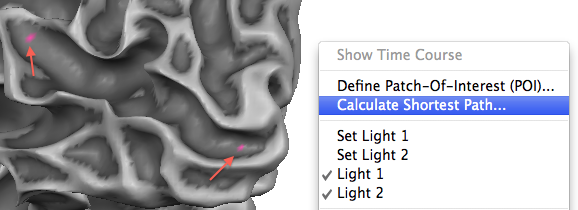
Since BrainVoyager QX 2.4 a special tool is available to calculate shortest paths and short paths that fullfill additional constraints. This tool can be invoked from the context menu of the surface rendering window that can itself be invoked by holding the right mouse button (or the appropriate means to signal a right mouse / context menu event); note that the context menu does not appear immediately but only after about a second since the right mouse button is also used for navigation in the mesh scene. The first and last vertex of the desired path can be defined by clicking at two desired locations before entering the Shortest Path dialog or - if known - by directly entering their indices in the From vertex and To vertex text boxes in the Shortest Path dialog (see snapshot below).
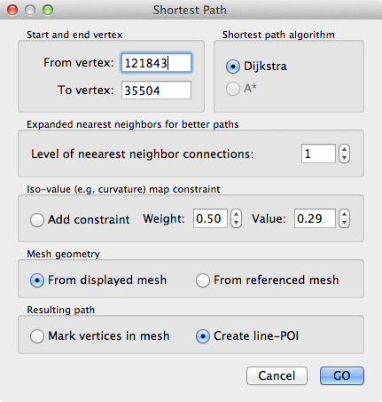
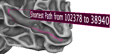
Keeping the default settings when clicking the GO button, the shortest path between the start and end vertex will be calculated using the Dijkstra algorithm using the vertex distances of the displayed mesh; the returned shortest path is the set of vertices connecting the start vertex to the end vertex via those direct neighbors that produce the smallest sum of vertex-vertex distance values. The resulting path will be visualized as a POI path (see below). Note that the length of the calculated shortest path will be printed in the Log pane, e.g. for the example used, the following text will be displayed:
Length of calculated shortest path between vertex 102378 and vertex 38940: 51.8038
Note that the "shortest" path depends on the directions that are locally possible when moving from a vertex to one of its nearest neighbors. Including not only the direct nearest neighbors but also the neighbors of the neighbors will produce smoother and shorter paths that are closer to "ideal" paths. In order to use both direct neighbors as well as neighbors of the direct neighbors to create a shortest path, the Level of nearest neighbor connections spin box in the Expanded nearest neighbors for better paths field can be changed from "1" (default) to "2". higher indirect neighbors than level 2 are not possilbe since the improvement is already substantial and using more indirect neighbor levels may lead to "short cuts" that are not desirable. With the default setting From displayed mesh the path uses the geometry of the mesh as displayed. If one visualizes a folded or flattened cortex mesh, i.e. to more easily specify the begin and end of a path, but one wants to calculate the shortest path on a referenced folded mesh, the From referenced mesh option need to be turned on in the Mesh geometry field.
Creation of Shortest Paths with Additional Constraints
While calculating the shortest path (geodesic) between two vertices on a folded mesh is useful to measure distances along the cortex, it is useful for some applications to add additional constraints when constructing a desired path. The shortest path tool allows to add such a constraint using values from a available surface map (SMP). One particularly useful map is a curvature map since it can be used to constrain paths to run along the fundus of a sulcus (highest concave curvature values) or along the crown of a gyrus. While the usage of the map constraint is exemplified below for labeling sulci using a curvature map, it is important to realize that any surface map can be used as constraint. Note that the shortest path tool will always use the first sub-map in case that several sub-maps are available.
A curvature map can be calculated by clicking the Curvature button in the Calculate curvature field of the Background And Curvature Colors dialog. To check that the curvature map is the only (or first) sub-map, the Surface Maps dialog can be used. Note that the Shortest Path dialog keeps the two vertices for the begin and end of a path, i.e. you need not to re-click on these vertices when calculating a new path between the same vertices but with different constraints. When re-entering the dialog, make sure that the Add constraint option in the Iso-value (e.g. curvature) map constraint field is turned on. The Weight spin box contains a relative weighting value w specifying how strong the additional map constraint should be used in relation to the pure path length constraint pl; the cost function c is calculated as c = w*abs(mv - mref) + (1-w)*pl. Here mv is the map value of the currently considered vertex v while mref is the reference map value specified in the Value spin box of the Iso-value (e.g. curvature) map constraint field. Note that this value is set to the map value of the start vertex when opening the Shortest Path dialog but it can be set to any desired value. Since a better cost function corresponds to lower values of the cost function, the values mv and mref should be more similar for a vertex on a preferred path than on alternative paths. Note that when using the map constraint, the Log pane does not print a path length value but the cost value c of the respective path. In order to obtain the length of a POI path use the Measure button in the POI path functions field of the Edit Patch-Of-Interest (POI) dialog.
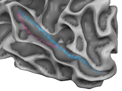
Since the (absolute) curvature values are usually highest at the fundus of a sulcus, the Value entry should be set to a value close to the largest value within the sulcus. Since the begin vertex will be selected in the fundus of a sulcus, it reflects often already a good map value for the labeling purpose; even better results may be eventually obtained by setting a slightly higher value that is close to (or larger than) the level of the maximum map value within the desired path. In the snapshot above, the blue path was created using the curvature map constraint and it is evident that the path runs more through the middle of the sulcus as opposed to the shortest path (magenta colored vertices).
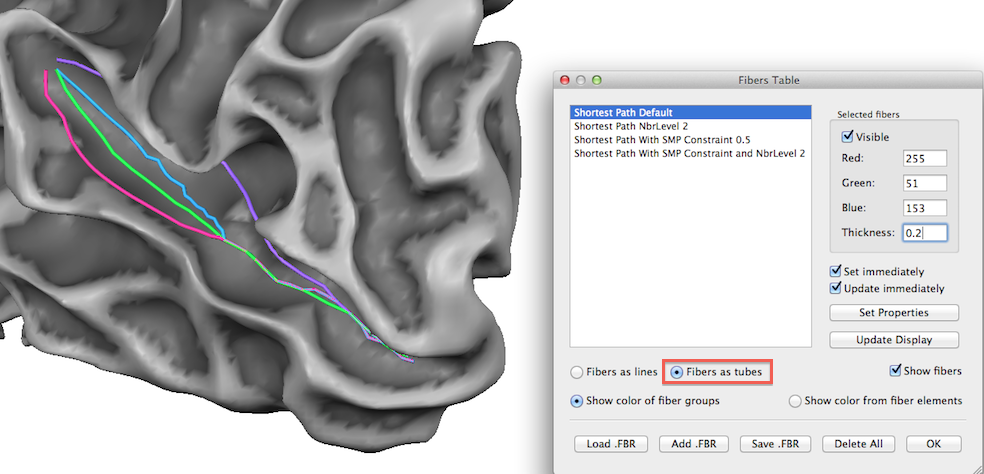
As described in the POI Path Tools topic, a POI path can be visualized as a 3D line or tube in the same way as a fiber track. The snapshot above shows the two paths from the previous image rendered as tubes; furthermore two additional paths are visualized that are defined in the same way as the previous path but usin a neighbor level of 2. The best results for the labeling purpose is achieved by the green path that uses neighbor level 2 and the (curvature) map constraint.
Copyright © 2014 Rainer Goebel. All rights reserved.