BrainVoyager QX v2.8
Cross-Correlation Analysis of Phase-Encoded Stimuli
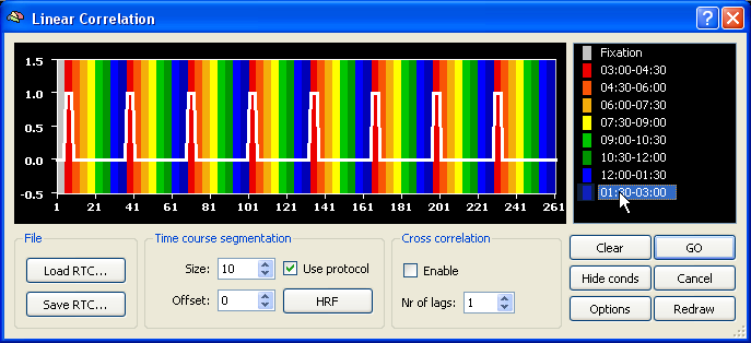
In order to map visual space to corresponding regions in the visual cortex with standard dynamic checkerboard stimuli, cross-correlation analysis can be used identifying the time point (lag) at which a region responds maximally. A mathematically identical approach consists in calculating the phase value at each voxel in the context of a Fourier analysis (available in a later release). In order to run a cross-correlation analysis, invoke the Linear Correlation dialog from the Analysis menu. In the example data below, 8 repetitions of one eccentricity (expanding annulus) or polar angle (rotating wedge) cycle has been conducted. The polar angle mapping experiment started with a wedge at 3 o'clock and rotated clockwise. Each expansion (from the minimal to the maximum size) or wedge rotation (once around the clock) lasted exactly 32 measurements (TR=2000 ms). In the defined protocol, each expansion/rotation cycle was divided into 8 segments each containing 4 measurements. In order to define the reference function for the correlation analysis, click with the right mouse button on the first (red colored) condition, and with the left mouse button at all other conditions. This will create a reference function similar to the one shown below.
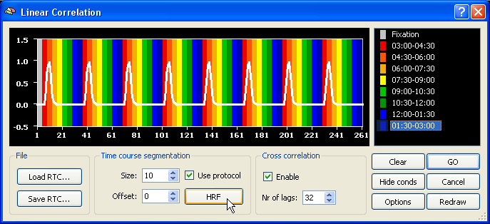
In order to get a hemodynamically convolved reference function (see figure below), click the HRF button. The defined reference function would only correlate high with voxel time courses, which were activated at the beginning of each (eccenricity or polar) cycle. In order to find also voxels responding at other moments within a cycle, the reference function has to be shifted to the right. A cross-correlation performs such shifts and calculates as many correlation values as there are shifted copies of the original reference function. The number of shifts is specified as the number of "lags" in the context of cross-correlation. Since one complete circle in our sample data consisted of 32 time points, specify the value "32" in the Nr of lags field within the Cross correlation field. Make sure also that the Enable option has been checked.
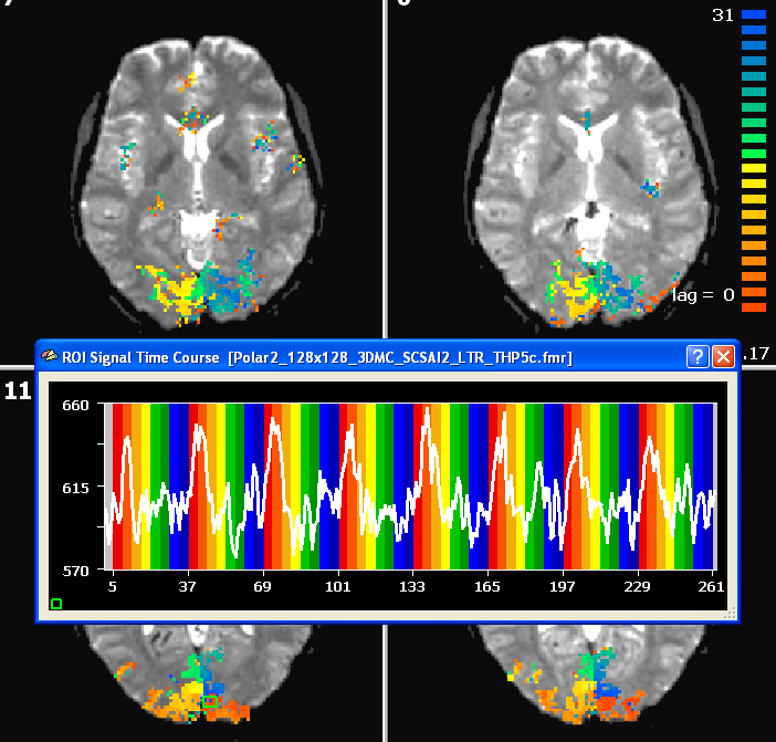
After clicking the GO button, the specified reference function is correlated 32 times at each voxel resulting in 32 correlation values. The program does not store, however, 32 correlation values per voxel but selects the maximum correlation value together with the lag (shift) at which the maximum correlation was obtained. When visualizing the resulting statistical map, you can chose to see either the maximum correlation value map or the lag map. The lag map is more important because it visualizes the moments within a cycle when a certain voxel correlated best and thus indicates to what eccentricity or polar angle the voxel responds.
The figure below shows the result of a cross-correlation study of the polar angle mapping experiment analyzed using the FMR data. In this example, functional data was obtained using 28 slices with 1.8mm x 1.8mm x 1.8mm voxels (128 x 128 matrix, TR = 2000 ms). The time course shown stems from a foveal region from slice 11.
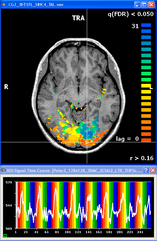
After creating a VTC file for the eccentricity and polar angle data, the same cross-correlation analysis can be performed in Talairach space. The snapshot shows an axial slice with the resulting polar angle lag map and a time course of a foveal region.
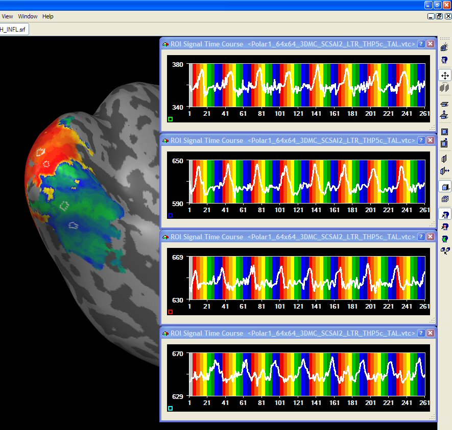
After having prepared inflated and flattened cortex representations of the subject's brain, the cross-correlation analysis can also be performed and visualized on the cortex. You may either project the calculated volume (VMP) maps on the cortex using the Create Map button in the Surface Maps dialog. Alternatively, you may want to bring the time course data first completely on the cortex creating MTC files and then run the cross-correlation anaysis on the MTC data. The figure below shows the polar angle lag map on an inflated cortical hemisphere. Since inflated and flattened cortex representations show topological order along the cortex, the visual-field specific response pattern ("stripes") is much more clearly visible than in the VMR-VTC-VMP analysis.
In order to improve the visualization on a cortical mesh, slight smoothing along the cortex is helpful. This can be done by entering the Surface Maps dialog. Make sure that the surface map is selected in the SMP list and then enter the Options dialog by pressing the Options button. In the Options dialog, you may click the Smooth SMP button. In order to only produce modest smoothing, select "3" (instead of default "5") smoothing iterations.
Copyright © 2014 Rainer Goebel. All rights reserved.