BrainVoyager QX v2.8
Mapping Local Pattern Information with a Multivariate Searchlight
Background
As described in previous topics, SVM classifiers can be applied to ROIs as small as a few voxels up to ROIs encompassing the whole brain. When using very large ROIs, a huge amount of features (voxels) is included in distributed patterns for trials and a classifier might not produce high generalization accuracies because of too many "noise" voxels. Recursive feature elimination helps to some extent to reduce the "curse of dimensionality" problem. Another popular approach to look in the whole brain for discriminative pattern information is provided by the searchlight mapping approach (Kriegeskorte, Goebel, Bandettini, 2006). In this approach, each voxel is visited, as in a standard univariate analysis, but instead of using only data of the visited voxel for analysis, several voxels in the neighborhood are included forming a set of features for joined multivariate analysis. The neighborhood is usually defined roughly as a sphere, i.e. voxels within a certain (Euclidean) distance from the visited voxel are included. The result of the multivariate analysis is then stored at the visited voxel (e.g. a t value resulting from a multivariate statistical comparison or an accurracy value from a support vector machine classifier). By visiting all voxels and analyzing their respective (partially overlapping) neighborhoods, one obtains a whole-brain map in the same way as when running univariate statistics. Since the performed multivariate analysis operates with voxels in a neighborhood, this approach is also called local pattern effects mapping.
Application
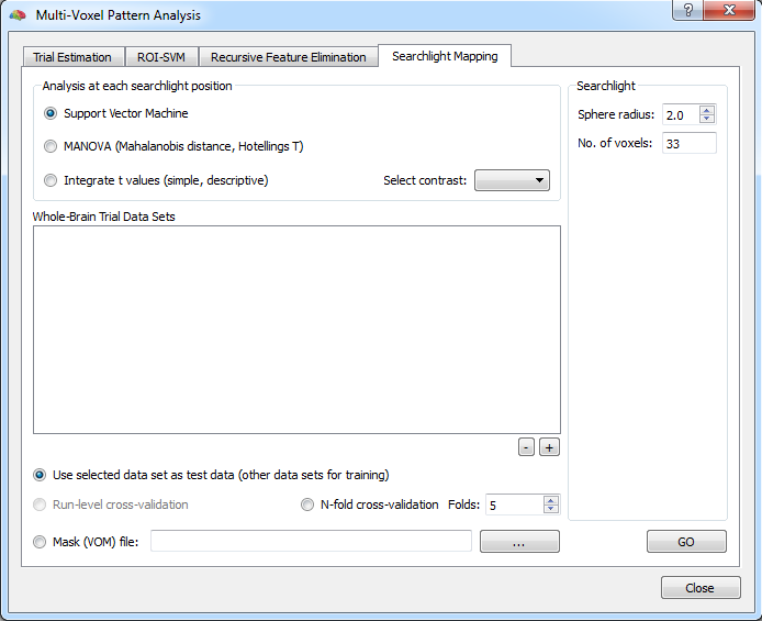
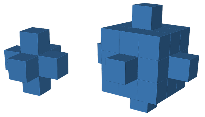
In order to use the searchlight tools in BrainVoyager, open the Multi-Voxel Pattern Analysis dialog and switch to the Searchlight Mapping tab (see snapshot above). The common feature of the searchlight approach is that a 3D "sphere" (a voxelated region of a certain size) is moved to each voxel for local pattern effects analysis. The Sphere radius spin box in the Searchlight section can be used to define the size of the sphere. Voxels in the neighborhood of a current (central) voxel are included, if their Eucledean distance is equal or less than the value provided in the Sphere radius field. The snapshot on top of this topic shows the 3D shape of the voxelated spheres for radius "1" and radius "2". Note that you can also enter non-integral values, such as 1.7 in the radius field to produce more compact spheres. Note that the coordinates of voxels included in the voxelated sphere ROI for a specified radius are printed in the Log pane relative to a central voxel with coordinates x=0, y=0, z=0.
While the specified radius defines the shape of the sphere that is moved around, different multivariate analysis approaches can be selected to be performed within each searchlight at each voxel location:
- Support Vector Machine (SVM) classifier
- Multivariate t test (Hotellings T)
- A simple descriptive method integrating squared t values
The first two methods are available since version 2.6 while the simple descriptive method is available since version 2.0. As a current limitation, the SVM and MANOVA searchlight tools can only handle two-class problems at present. If you have multi-class trial-estimation data sets, you may either delete trial volumes in the Volume Maps dialog or rerun trial estimation including only two classes.
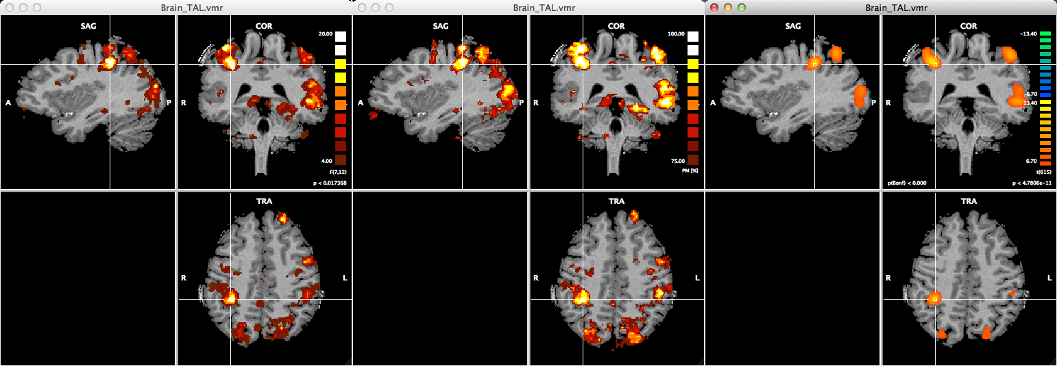
The snapshot above shows a comparison of the results obtained with the three different searchlight analysis methods using the same data set. The left VMR view shows an overlaid F map resulting from a MANOVA searchlight, the middle VMR view shows an overlaid cross-validated accurracy map resulting from the SVM searchlight, and the right VMR view shows an overlaid descriptive t-integation F map. While the intention is usually to run searchlight classifiers over the whole-brain, the SVM and MANOVA searchlight analyses can also be restricted to a mask that needs to be provided by a prepared VOM file. If you have a VOI defined as a mask, you need to convert the corresponding .voi file first into a .vom file. If availalbe and desired, the .vom file can then be selected using the Browse ("...") button at the bottom of the Searchlight Mapping tab; selecting a .vom file will automatically turn on the Mask (VOM) file option.
SVM Searchlight
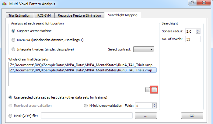
In order to use SVM-based searchlight mapping, select the Support Vector Machine option (default) in the Analysis at each searchlight position field. Use the + button below the Whole-brain trial data sets field to add VMP data sets containing single trial estimates for all voxels of the scanned volume (usually whole-brain data). Consult the trial estimation topic to learn how to create trial estimates for each voxel serving as input for training classifiers. To assess whether a classifier has learned to discriminate between distributed patterns of different conditions, test data needs to be availalbe that was not used during training. One way to specify test data is to select one VMP data set as test data set and all others as training data set. To select the test data set, click the respective VMP data set in the Whole-brain trial data sets list and turn on the Use selected data set as test data option. In the snapshot below this option is checked and the "RunB_TAL_Trials.vmp" file is selected implying that the "RunA_TAL_Trials.vmp" file is used for training.
MANOVA Searchlight
Integrating t Values Searchlight
To select the integrating univariate t values approach, check the Integrate t values (simple, descriptive) option. This analysis appraoch is a simple method to quickly obtain a map showing regions with differential information content. This method uses the t values obtained from a standard univariate contrast map that are combined within a sphere in such a way that positive and negative t values do not cancel out. One way to do this is to use the sum of the absolute t values within the searchlight, another way that is used in BrainVoyager is to sum the squared t values. Note that this simple analysis approach should only be used for descriptive information-based mapping (Kriegeskorte and Bandettini, 2007). To use this searchlight analysis approach, at least one contrast map needs to be calculated, e.g. using the standard Overlay GLM Contrasts dialog to specify a GLM contrast between two conditions after running a GLM analysis (using little or non-smoothed functional data). All available contrast maps (usually one) appear in the Select contrast combo box on the right side of the Integrate t values option. Select the contrast you are interested in (or keep the default selection in case of one available contrast) and click the GO button to start the analysis. Because of the simple calculations necessary for this approach, the resulting map will be visualized already after a few seconds.
Note that averaging the squared/absolute t-values within a voxel's spotlight is equivalent to a searchlight mapping using the Euclidean distance as the multivariate effect measure that indicates the difference between the activity patterns within the searchlight. If error covariance among searchlight voxels is to be taken into account, the Euclidean distance is replaced by the Mahalanobis distance (Kriegeskorte et al. 2006) that is used in the MANOVA searchlight approach (see above).
References
Kriegeskorte, N., Goebel, R., & Bandettini, P. (2006). Information-based functional brain mapping. PNAS USA, 103, 3863-3868.
Kriegeskorte, N. & Bandettini, P. (2007). Analyzing for information, not activation, to exploit high-resolution fMRI. NeuroImage, 38, 649-662.
Copyright © 2014 Rainer Goebel. All rights reserved.