BrainVoyager QX v2.8
Intensity Inhomogeneity Correction
Background
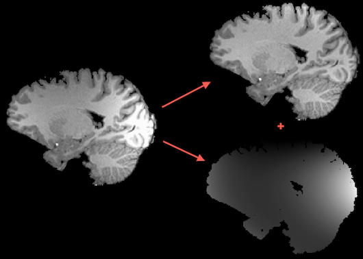
Intensity inhomogeneities in MR images can substantially reduce the accuracy of segmentation and registration. Despite advances of correcting spatial intensity inhomogeneities of modern scanner software, the advent of multichannel phased array coils and 7T+ scanners have increased (again) the importance of this problem for post-scan processing since images may exhibit substantial intensity inhomogeneities across space (see image on left side in figure above). This poses a problem for segmentation tools that are based on region growing approaches since white matter voxels at one position of the image might have the same intensity as grey matter voxels at other locations in the image. One well-performing method of intensity inhomogeneity correction (IIHC) that compares well with other methods (e.g. Sled et al., 1997) is based on a "surface fitting" approach. In this approach, low-order polynomials are used to model low-frequency variations across 3D image space; these polynomials are fitted to a subset of voxels that have been labeled as belonging to white matter. After estimating the low-frequency intensity fluctuations (producing a "bias field", see image on lower right side above), they are removed from the data producing voxels with much more homogeneous intensities (see image on upper right side above) that improve visualization and also are better starting points for subsequent segmentation tools.
In BrainVoyager QX 2.1 and earlier it was necessary to select presumed white matter voxels using region growing in specific intensity ranges. This manual "pre-segmentation" step is often time-consuming since several attempts are usually required until good intensity range values are found; furthermore, the obtained quality depends on the experience of the user. Version 2.2 of BrainVoyager QX introduced a new IIHC tool that contains as its core the same polynomial "surface fitting" approach but includes new tools that allow to run IIHC without user intervention. Since bias field estimation works more precise when it's focused on brain tissue only, a background cleaning step followed by a brain extraction step are useful preparator steps. More specifically, BrainVoyager QX executes the following steps during automatic intensity inhomogeneity correction:
- Background cleaning. The background is cleaned, i.e. intensity values of voxels in the background are set to zero. This is performed by determining the voxels with lowest intensities in a V16 intensity histogram and those voxels are then set to 0 intensity. Due to variability in background voxel intensities, this step will not set all voxels in the background to 0 but "salt'n pepper" noise will remain. To clean the background further, the 3D VMR image is binarized, i.e. all intensity values larger than 0 are set to the same integral value (while value "1" would be fine, BrainVoyager uses value 240 since this is vsualized as "blue" in a VMR whereas value 1 would be not visible since it would be visualized as black). On the binarized image, the largest connected component is determined and all other components are set to 0. Since the head/brain constitutes a much larger component than the clusters in the background, the head/brain will be remaining but the background voxels are removed. The "surviving" component is saved as a VMR file to disk under the name "[orig-name]_HeadMask.vmr" and this file is used as a mask file for the V16 data.
- Brain extraction. The brain is extracted from the cleaned VMR using again a binary representation of the VMR data and morphological operations. First the binary image is eroded in order to break intensity connections between the brain and the surrounding head tissue. This is followed by determination of the largest connected component that is retained while all other components are set to 0. Since the brain is usually the largest component after erosion, a "shrunken" version of the brain is extracted at this point. In order to re-add the fringe of the brain, the performed erosion step is inverted using a dilation operation. The resulting component is saved as a VMR file to disk under the name "[orig-name]_BrainMask.vm" and this file is used as a mask file for the V16 data (if this file is not available, the "HeadMask.vmr" is used).
These preparatory steps are executed once and only if the respective mask files are not available; if the mask files are located in the folder of the original file, they will be automatically applied and the preparatory steps will be disabled. The subsequent steps are performed repeatedly, usually twice. - White matter detection. After brain extraction, the voxels with highest intensities should reflect white matter voxels; due to the spatial inhomogeneities it is, however, not appropriate to simply select the voxels with high intensity values since grey matter voxels in bright spots of the image (high signal-to-noise) might have higher intensity values than white matter voxels in "dark spots" (lower signal-to-noise). In order to detect white matter voxels, BrainVoyager selects the highest intensity values within local data blocks with N = 5 x 5 x 5 = 125 voxels. Furthermore it heuristically checks whether the intensity distribution within a local block stem from one or two tissue types. The latter check is performed using the trimmed range statistic (e.g. Hou et al., 2006); first the intensitye values are ranked in increasing order xi (more precisely in non-decreasing order since some voxels may have the same intensity values); each value is then divided by 2 times the median of the local distribution: yi = xi/(2 XN/2) . With these normalized values, the trimmed range statistic can be calculated for 1 < j < k < N as r = yk - yj (with j = 2 and k = N-1 in current implementation). If the trimmed range is smaller than a specified tissue range threshold (default: 0.25) than it is assumed that the intensities in the local block stem from only one tissue type and only those homogeneous blocks are considered further, i.e. blocks with presumed multiple tissue types are not included in white matter detection. The medians of the identified homogeneous blocks are then ranked in increasing order and a specified percentile (default: 30%) of blocks with low median intensities is discarded. The voxels in the surviving blocks are labeled as white matter candidates. While this heuristic does not guarantee a correct separation of white and great matter voxels, the likelihood is very high that a large sub-part of white matter voxels is included in the ramaining set of voxels. Repeating the process will further increase the validity of white matter labeling.
- Bias field estimation within white matter voxels. The labelled white matter voxels serve as "seed points" to fit (using svd-based least squares) low-order (Legendre) polynomials to capture how white matter intensities vary across 3D image space; the default order of polynomials is set to "3" usually providing excellent results. The estimated parameters of the polynomials are used to construct the bias field that is finally removed from the V16 data set.
The "White matter detection" and "Bias field estimation" step may be executed repeatedly (default: 2 times). The separation of white and grey matter is indicated by plotting a intensity histogram at each iteration. The resulting V16 data set is finally converted to a VMR data set; if specified (default: yes), grey matter intensities will be centered around intensity "100" and white matter intensities around "160".
Running Automatic IIHC
The described steps are available in the 16 Bit 3D Tools dialog (see below) that can be invoked using the Volumes > Inhomogeneity Correction, V16 Tools menu item. Note that the .v16 data set belonging to the .vmr data set (i.e. a file with the same name as the current VMR but with extension .v16) is automatically loaded if it can be located in the same folder, otherwise the Load .V16 button can be used to load an appropriate V16 file.
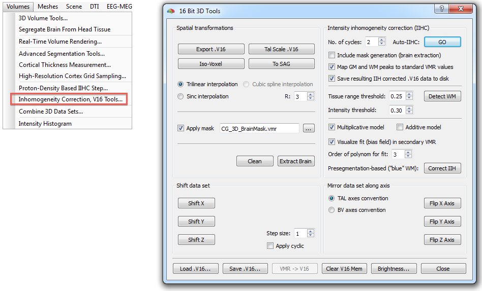
In most cases, pressing the GO button (see snapshot above) in the Intensity inhomogeneity correction (IIHC) field is sufficient to create a homogeneous data set in a few seconds. Starting the automatic IIHC tool triggers the sequence of processing steps described above resulting usually in a segmented, homogeneous brain data set (see top right image in figure of Background section above and right image in snapshot below). The preparatory steps option, Include mask generation, can be turned on or off; it is automatically checked in case that this step has not yet been performed (i.e. if no "_MaskBrain.vmr" file is availalbe in the folder of the VMR/V16 file). If the Map GM and WM peaks to standard VMR values is turned on (default), the grey matter and white matter intensities will be centered around intensiy values of 100 and 160, respectively. Detection of white matter can be influenced by changing the Tissue range threshold and Intensity threshold (percentile of low intensity homogeneous blocks) values, for details, see description above. The order of the Legendre polynomials can be set in the Order of polynom for fit option (default: 3). When the Save resulting IIH corrected .V16 data to disk option is checked (default), the resulting IIHC corrected V16 file will be saved to disk.
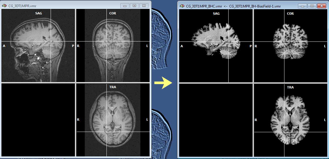
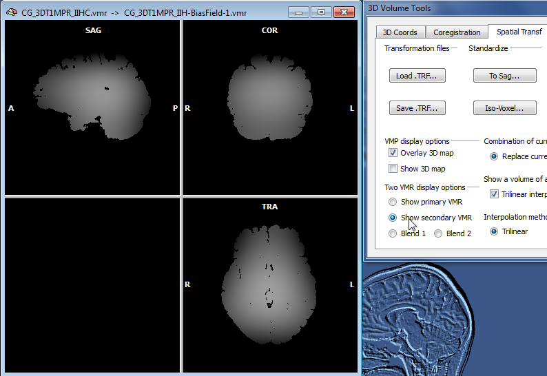
The snapshot above shows the result of IIHC for a 3D data set with only rather small inhomogeneities (left), nonetheless the resulting data set indicates a gain in white and grey matter separation and within-tissue homogeneity. Note that BrainVoyager stores the resulting file under the name of the original VMR/V16 data set but with the substring "_IIHC" (see title bar of window on right side in snapshot above). In addition to an inhomogeneity corrected VMR/V16 data set, the automatic procedure also generates representations of the generated bias fields. A bias field represents the fitted model of the low-frequency intensity variations of the automatically labeled white matter voxels over space (see bias field image below).The estimated bias fields are also stored to disk using the name of the original file plus the substring "_IIH-BiasField[nr]" where the "[nr]" part refers to the iteration of the IIHC process. Since the first calculated bias field highlights the most severe inhomogeneities, it is shown as default in the secondary VMR of the corrected VMR view even when running multiple iterations. Bias field visualizations from subsequent iterations can be loaded as separate (primary) VMRs or loaded in the secondary VMR view. To visualize the produced bias field, the usual 1st / 2nd volume toggle key (F8) can be used or the Show primary VMR / Show secondary VMR options in the Two VMR display options field in the Spatial Transf tab of the 3D Volume Tools dialog (see snapshot below).
While a single run of the automatic IIHC process leads to very good results, the process is repeated once as default (No. of cycles: 2) in order to further increase the resulting homogeneity. More than two iterations do usually not lead to significant further improvements as can be assessed with the displayed intensity histograms that are generated for each iteration (see figure below). Each histogram shows the result before (blue line) and after (yellow line) application of one cycle through the processing pipeline. In the plot on the left side below (iteration 1), the blue line indicates that white and grey matter voxel intensities overlap substantially since there is only one broad peak in the histogram; the yellow line indicates the successful application of the automatic inhomogeneity correction process clearly revealing two peaks corresponding to grey and white matter. After the second iteration (snapshot below, right side) not much further improvement is visible.

While IIHC can be executed automatically clicking the GO button, all involved steps can also be used in isolation, including background cleaning (Clean button), brain extraction (Extract Brain button), white matter detection (Detect WM button) and bias field estimation and removal (Correct IIH button). Separate execution with non-standard parameters may be useful in rare cases where the automatic process does not lead to satisfactory results; while the default setting of these parameters are usually working well, it might be useful to change them in specific situations.
Tip: For visualization purposes, within-tissue homogeneity can be further enhanced by running the Sigma filter from the Filter, smoothing field in the Segmentation tab of the 3D Volume Tools dialog. If one plans to run (advanced) segmentation tools subsequently, this step should not be performed since it is executed as part of automtic segmentation routines.
References
Hou, Z, Huang, S, Hu, Q, Nowinski, WL (2006). A fast and automatic method to correct intensity inhomogeneity in MR brain images. In: R. Larsen, M. Nielsen, and J. Sporring (Eds.): MICCAI 2006, LNCS 4191, pp. 324–331, Springer: Berlin, Heidelberg.
Sled (1997). A comparison of retrospective intensity non-uniformity correction methods for MRI. Lecture Notes in Computer Science.
Copyright © 2014 Rainer Goebel. All rights reserved.