BrainVoyager QX v2.8
Preparatory Steps
High-Resolution Iso-Voxel Data
Since high-resolution structural data sets are important for advanced segmentation and cortical thickness measurements, the advanced segmentation tools support structural data sets of arbitrary (sub-millimeter) resolution and dimensions beyond 256. If available, sub-millimeter data sets measured at sub-millimeter resolution should be used as input for advanced segmentation. If only 1 mm (standard) resolution is available, the Advanced Segmentation Tools dialog recommends to upscale the voxels to 0.5 mm resolution as a first preparatory step.
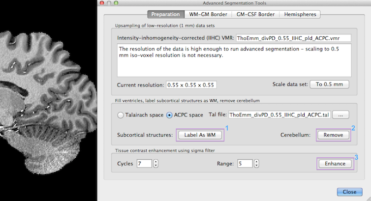
Since BrainVoyager QX 2.8, the program advises in the Resolution text field in the upper section of the Preparation tab whether upsampling should be performed or not. Since the example data set used above has a resolution of 0.55 mm iso-voxel acquisition resolution, no upscaling is required (7 Tesla data courtesy of Thomas Emmerling, Maastricht University). In previous versions, some functions (like subcortical masking avoiding manual editing) were only available if the input data was prepared in 1 mm ACPC or Talairach space. These preparatory tools now also work for ACPC and Talairach transformed sub-millimeter data sets. Note that the (sub-millimeter) data sets should be brought in ACPC or Talairach space using sinc or cubic spline interplation. If this has not been done with your data set, you may rerun the transformation by using the re-apply spatial transformation tool, which is available in the VMR Properties dialog. You can also use data sets in sub-millimeter native (non-ACPC/TAL) space but then the subcortical masking tools will not work.
In case that only 1 mm - high-quality - data sets are available, the To 0.5 mm button in the Updampling low (1mm) resolution data sets field can be used. This will invoke the Iso-Voxel Transformation dialog with appropriate settings. You may simply click the OK button to start the spatial transformation (scaling operation). Because it is important to retain the data quality as much as possible, only sinc or cubic spline interpolation should be used. Sinc interpolation may run slow on standard CPUs but a fast version is available that exploits modern graphics cards. Note that the dimensions of the data are internally transformed from 256 to 512, which results in a data set requiring 8-fold working memory (2 x 2 x 2). To reduce working memory load as well as storage space, the dimensions of the obtained 0.5 mm data are minimized to capture only those voxels in a sub-cube, which actually contains data (non-zero values). This "minimized cube" operation should also be performed for true sub-millimeter data sets using the Minimize button in the VMR Properties Options dialog. This operation adds offsets to the VMR headers and also keeps infromation about the original embedding space (the "framing cube dimensions"). An example data set before and after upsampling is shown in the snapshot below.
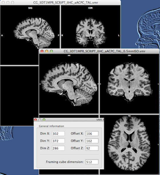
You can see that the resulting 0.5 mm data set (see snapshot above) does not have much "empty" space around the brain as compared to the original data set. The newly created VMR also gets a new extension substring "_0.5mmISO" to indicate the performed upscale transformation. Since the program needs to know the true voxel positions, offset values for each dimension are stored with each VMR (similar as with VTCs and VMPs). If you open the VMR Properties dialog of the 0.5 mm VMR, you will see these new offset entries in the General information field (see inset in snapshot above).
Removal of Subcortical Structures and Cerebellum
The next preparatory step consists in identifying the shape of the ventricles in the brain as well as the location of subcortical structures. These steps are at present performed in the same way as described in section Mask-Based Removal of Non-Cortical Structures except that they are adjusted to work correctly with any sub-millimeter resolution ACPC and Talairach data sets (since BrainVoyager QX 2.8). To enable resolution-independent masking operations, the program creates proper masking data from a standard 0.5mm Talairach space mask file that is placed in the folder containing the BrainVoyager QX executable during software installation; this mask file is resampled to the resolution of the input data set. In case that the current data is in ACPC space, the Talairach landmark (TAL) file needs to be provided in the Fill ventricles, label subcortical structures as WM, remove cerebellum field (see snapshot below). With the proper TAL file, the mask is resampled to the resolution of the data set followed by an inverse Talairach ("Un-TAL") transformation.
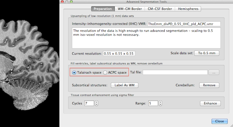
Since the used example 0.55 mm data set resides in ACPC space, the ACPC space option has been selected and the Talairach file has been provided in the snapshot below.
After clicking the Label As WM button in the Fill ventricles, label subcortical structures as WM, remove cerebellum field, the identified ventricel and subcortical structures are "removed" by labelling them as white matter as indicated in the snapshot below. The identified structures are set to an intensity value of 225 (white).
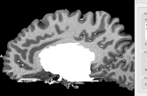
This preparatory step is completed by removing (large parts of) the cerebellum as well as the spinal cord. After clicking the Remove button in the Fill ventricles, label subcortical structures as WM, remove cerebellum field, the resulting data set should look similar as shown in the snapshot above.
Enhancement of Tissue Contrast and Homogeneity
The final preparatory step works similar as described in section Tissue Contrast Enhancement. It uses a sigma filter to enhance contrast between tissue types by smoothing intensity values around each voxel while taking care that only voxels are included in this process containing intensity values with values close to the intensity of a considered voxel. Limiting smoothing in that way increases the likelihood that smoothing acts only within tissue types without spreading across boundaries to other tissue types resulting in overall contrast enhancement. This step profits substantially from sub-millimeter resolution since smoothing across tissue boundaries is better restricted than with a 1 mm voxel resolution.
It is recommended to keep the default setting of 7 cycles in the Cycles spin box and an inclusion range of 5 intensity levels in the Range spin box (see snapshot above) but if you obtain non-optimal results, you might want to change these values, especially the Range value. Note, however, that your data might not be suited for advanced segmentation if you do not see borders as least as clear as shown in the figure below. To start the process, click the Enhance button in the Tissue contrast enhancement using sigma filter field.
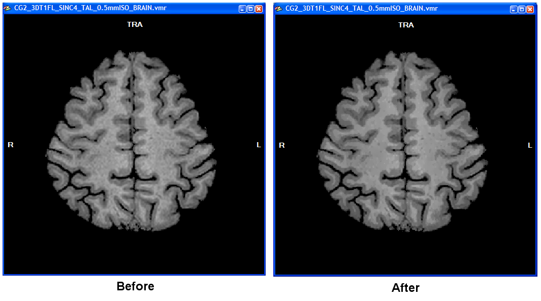
The computation will last a few minutes. A dialog will inform about the progress made. In the resulting data set it is much easier to see the WM-GM boundary (right side of figure above) as compared to the unprocessed data set (left side in figure above). Note that the data shown above is from a rather low 1mm data set that was upscaled to 0.5 mm. In case you are using acquired sub-millimeter data of high-quality as shown in the 0.55 mm 7 Tesla example data, you may not see much improvement since the two tissue types are already rather homogenous and separated from each other by clear intensity "jumps".
The data set is now prepared for segmentation of the white / grey matter boundary.
Copyright © 2014 Rainer Goebel. All rights reserved.