BrainVoyager QX v2.8
Measuring Cortical Thickness in Volume Space
Cortical thickness measurement requires as input a structural (VMR) file, which has been successfully segmented using the advanced segmentation tools. The result of the advanced segmentation procedure is a file with a name like "<initial_string>_0.5mmISO_BRAIN_WM_GM.vmr" containing both the WM / GM boundary and the GM / CSF boundary. After loading this file, you can launch the Cortical Thickness Measurement dialog (see below) by clicking the Cortical Thickness Measurement item in the Volumes menu.
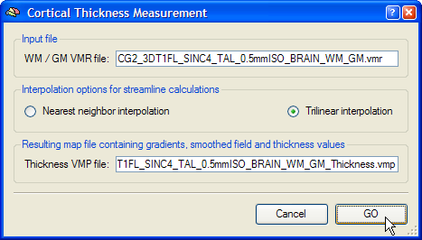
The name of the loaded VMR file with the WM / GM and GM / CSF boundaries will appear in the WM / fGM VMR file field. The Interpolation options for streamline calculations field allows to select either the Nearest neighbor interpolation or Trilinear interpolation (recommended) option for the computation of "streamlines" (see below). To measure cortical thickness, simply click the GO button. The result will be a volume map (VMP) file containing submaps with the cortical thickness estimates as well as other useful information. A name for the resulting VMP file is suggested in the Thickness VMP file text box.
The measurement of cortical thickness uses the Laplace method. After clicking the GO button, the following steps are performed:
- Three tissue classes are identified in the VMR file with respect to a voxel's intensity value i: CSF (i < 75), GM (75 ≤ i ≤ 125) and WM (i > 125 ). Before starting the main computations, these identified tissue classes are set to three intensity values: CSF: 50, GM: 100, WM: 150. The CSF and WM intensity values are not changed during subsequent computations ("border voltages"), only the intensities of GM voxels are updated incrementally. The starting intensity values are converted to real numbers (floats) in order to allow fine-grained calculations. The resulting volumes are stored as float volume maps (VMPs).
- The intensities of GM voxels are iteratively smoothed (200 iterations) in order to solve Laplace's equation. The resulting smoothed intensities are stored as map 4 ("Laplace smoothed") in the resulting VMP file (see figure below).
- At each voxel, gradient vectors are computed. Each gradient component (x, y, z) is saved in an individual map within the VMP file (maps 1 - 3, see figure below). While the gradient vector lenghts are normalized to 1.0 internally, the component values are saved multiplied by 10.0 in order to simplify thresholding for visualization purposes.
- For every GM voxel, a streamline is calculated using a small step size of 0.1. From a starting GM voxel, the gradient is first followed in one direction (i.e. "up") and then in the opposite direction (i.e. "down"). The integrated values of the accumulated step sizes until a boundary voxel is reached results in a pathlength. The pathlengths from the two directions are finally added together to obtain the thickness measure for the GM voxel. The computed thickness measures for all GM voxels are stored in map 5 ("Cortical Thickness") in the resulting VMP (see figure below).
After these calculations have been completed, the cortical thickness map (map 5) is shown superimposed on the VMR data. The VMP data structure resides in working memory but has been also saved to disk for later usage, especially for cortical thickness analysis in cortex space. Note that this file is very large (about 450 MB). If you click on Overlay Maps in the Analysis menu, the Volume Maps dialog appears with similar entries as shown in the snapshot below.
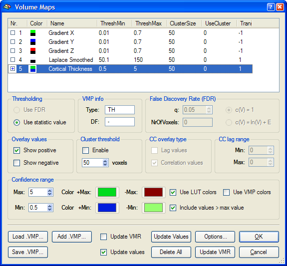
Note that the statistical look-up table has been automatically changed to better reflect the differences between thickness values as compared to the standard overlay colors. The program automatically loads the "Thickness.olt" look-up table from the folder "MapLUTs", which should be in your BrainVoyager QX folder after a regular installation. This look-up table shows thin cortex in blue and thick cortex in green. Since the computed maps have been saved to disk, you may superimpose the thickness map (or any other of the 5 maps) also on other VMR data sets of the subject, for example the original, unsegmented data.
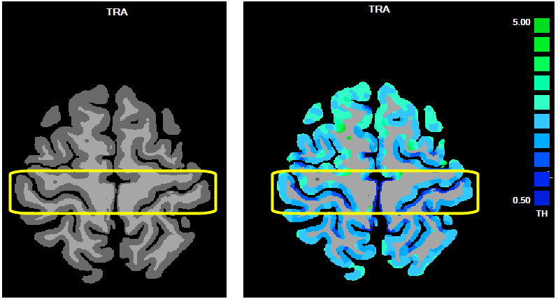
The figure above shows on the left side the input data set (result from the advanced segmentation tools) and on the right side the resulting cortical thickness map for a selected axial slice. The yellow box highlights regions around the central sulcus. It is known that the posterior bank of the central sulcus has a much thinner cortical thickness than the anterior bank. While this can be readily seen already in the segmented data (left side), the cortical thickness map (right side) quantifies this effect and the resulting values (anterior bank ca. 2.7, posterior bank ca. 1.8 ) are in accordance with the values reported in the literature. Since the central sulcus thickness values in the anterior and posterior bank differ substantially in individual brains, the values obtained there should be used as a check that the segmentation and thickness measurement procedures have worked satisfactorily. The effect is easily visible in the obtained cortical thickness map since the posterior bank contains mostly dark blue colors while the anterior bank contains mostly light blue and light green colors. The scale bar on the right shows the mapping from the colors to measured cortical thickness in millimeter.
Note: You can "probe" the cortical thickness measured at each voxel by moving the mouse across voxels and observing the thickness value in the status bar.
Copyright © 2014 Rainer Goebel. All rights reserved.