BrainVoyager QX v2.8
Adding High-Pass Filter Confound Predictors
As described in topic Temporal High-Pass Filtering in the Preprocessing chapter, low-frequency drifts can be either removed as a preprocessing step or as part of statistical data analysis. In the latter case, the design matrix will be extended by a set of confound predictors forming a Fourier or discrete cosine transform (DCT) basis set. Performing high-pass filtering by means of an extended design matrix has the advantage that statistical results are slightly more accurate as compared to performing it as a preprocessing step since the degrees-of-freedom will be adjusted for the number of added sines and cosines or DCT basis functions, respectively. This effect is, however, small due to the large number of time points in a typical functional run of 100 - 500 time points. A disadvantage of this approach is that other tools, e.g. event-related averaging will not work properly because they require stationary time courses. Furthermore, there are other preprocessing steps performed (e.g. motion correction) improving the data, which are not accounted for in the statistical data analysis. We therefore generally recommend to perform the high-pass filter as a preprocessing step except if there are specific reasons.
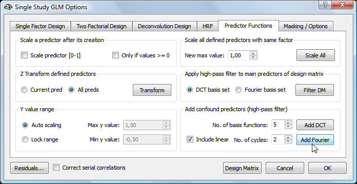
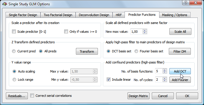
Before adding a high-pass filter, define the main predictors of the design matrix first. Then add a high-pass filter basis set using the options in the Add confound predictors (high-pass filter) field of the Predictor Functions tab of the Single Study GLM Options dialog.
Adding a Fourier Basis Set
One possibility is to use a Fourier basis set, which can be added by clicking the Add Fourier button (see snapshot below). The number of sine/cosine pairs can be adjusted by changing the value in the No. of cycles spin box. It is also advised to keep the Include linear option turned on. For details about the setting and interpretation of a Fourier basis set, consult the Temporal High-Pass Filtering topic.
The snapshot below shows the main predictors in color defined for the sample "Objects" experiment and the added predictors for the Fourier basis set in white.
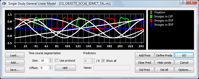
Another view of the predictors is obtained by clicking the Design Matrix button in the Single Study GLM Options dialog, which invokes the Design Matrix dialog (see below) showing a graphical view of the data. In this view, time is progressing from top to bottom with each column representing one predictor. The value of a predictor at a specific time point is shown as a grey value from black (value "-1") to white (value "+1"). The three main predictors are shown on the left side followed by the linear trend predictor, a sine/cosine pair with one cycle per time course and a sine/cosine pair with two cycles.

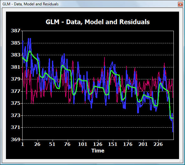
The snapshot below shows the time course from a selected region exhibiting a clear trend. Trends are visible in the VTC data since no high-pass filtering was applied during preprocessing. Despite of the trends, the statistical results for the main predictors are as good as those obtained after preprocessing the data - but only when adding the high-pass filter confound predictors.

The snapshot below shows how the selected time course (blue curve) is modeled using the design matrix (green curve) as the weighted sum of predictors of interest as well as predictors from the high-pass Fourier filter. Since the confound predictors remove the drift in the data, the beta values of the main predictors can be interpreted and compared.
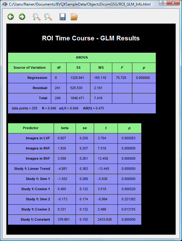
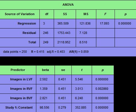
The detailed contribution of the predictors is revealed in the betas table shown below indicating that the drift is mainly "explained" by the linear trend predictor. Note that the confound predictors are only shown in the beta table if the Show confounds option is turned on in the ROI GLM Specifications dialog before clicking the Fit GLM button.
Adding a DCT Basis Set
As an alternative to a Fourier basis set, a discrete cosine transform (DCT) basis set can be used as a high-pass filter. To add a DCT basis set, click the Add DCT button in the Add confound predictors (high-pass filter) field of the Predictor Functions tab of the Single Study GLM Options dialog (see snapshot below). The number of included basis functions can be adjusted by changing the value in the No. of basis functions spin box. For details about the specification and interpretation of a DCT basis set, consult the Temporal High-Pass Filtering topic.
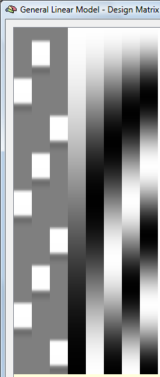
The resulting design matrix with the three main predictors and the DCT basis set is shown in the snapshot below, which is obtained by clicking the Design Matrix button in the Single Study GLM Options dialog. The three main predictors are shown on the left side followed by the five specified DCT basis functions.
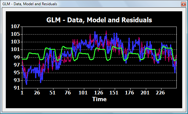
The snapshot below shows the time course of a voxel (blue curve) and how it is explained by the GLM (green curve).
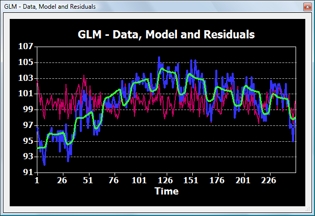
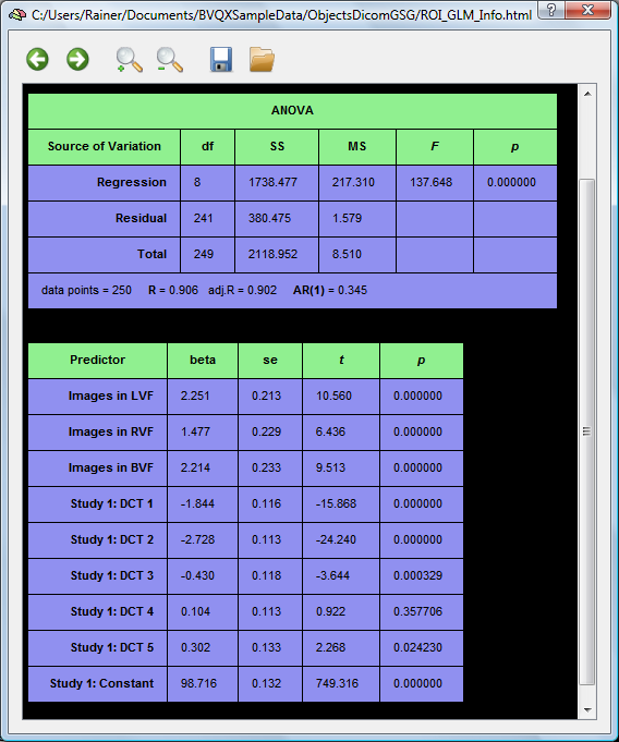
The beta values in the table below show that the non-linear drift in the time course is explained mainly by the first and second predictor of the DCT basis set (labelled "DCT 1" and "DCT 2"). Since the drift is explained by the high-pass filter, the betas of the main predictors ("Images in LVF/RVF/BVF" can be interpreted and compared using contrasts.
What would happen if the high-pass filter would not be included in the design matrix? The snapshot below shows that, as expected, the drift is not removed in this case. Is it safe to interpret and compare the beta values of the main predictors?
While in this example the relative pattern of the weights is quite similar as in the case with the high-pass filter, the interpretation of the weights is generally problematic. If, for example a linear drift occurs in the data and blocks of condition 1 always occur before blocks of condition 2, condition 2 will "benefit" from the trend if it increases from left to right, and condition 1 will benefit if the trend decreases from left to right. Even if two conditions would have the same amplitude, the trend might, thus, influence the estimated betas in such a way that a contrast between the two conditions might become significant. In order to avoid these problems, low-frequency drifts should be always removed, either as a preprocessing step (recommended) or during statistical analysis as shown in this topic.
Copyright © 2014 Rainer Goebel. All rights reserved.