BrainVoyager QX v2.8
Automatic ACPC and Talairach Transformation
The Talairach space is a common target space for normalization that is also closely related to the MNI space. In order to perform Talairach transformation automatically, two approaches are typically used: a) automatic detection of relevant landmarks and b) alignment to a template brain that has been previously transformed in Talairach or MNI space. The automatic Talairach procedure is described below and is currently the default brain normalization method in volume space (the template based alignment method will soon also be available in BrainVoyager). The next topic describes how Talairach transformation can be performed interactively by specifying relevant landmarks. It is helpful to read that topic because it is not only relevant in case that the automatic procedure is not applicable but it also provides more detailled knowledge about the individual steps involved in Talairach transfomation.
Background
In the original definition (Talairach & Tournaux, 1988), the midpoint of the anterior commissure (AC) is located first, serving as the origin of Talairach space. The brain is then rotated around the new origin (AC) so that the posterior commissure (PC) appears in the same axial plane as the anterior commissure. The connection of AC and PC in the middle of the brain forms the y-axis of the Talairach coordinate system. The x-axis runs from the left to the right hemisphere through AC. The z-axis runs from the inferior part of the brain to the superior part through AC. In order to further specify the x and z-axes, a y-z plane is rotated around the y (AC-PC) axis until it separates the left and right hemisphere (mid-sagittal plane). This completes the first part of Talairach transformation, often called AC-PC transformation. The obtained AC-PC space is attractive for individual clinical applications, especially presurgical mapping and neuronaviagation since it keeps the original size of the brain intact while providing a common orientation for each brain.
For a full Talairach transformation, a cuboid in AC-PC space is defined that runs parallel to the three axes defined in the first step enclosing precisely the cortex. This cuboid or bounding box requires specification of additional landmarks specifying the borders of the cerebrum. The bounding box is sub-divided by several sub-planes. The midsagittal y-z plane separates two sub-cuboids containing the left and right hemisphere, respectively. An axial (x-y) plane through the origin separates two sub-cuboids containing the space below and above the AC-PC plane. Two coronal (x-z) planes, one running through AC and one running through PC, separate three sub-cuboids; the first contains the anterior portion of the brain anterior to the AC, the second contains the space between AC and PC and the third contains the space posterior to PC. These planes separate 12 sub-cuboids. In a final Talairach transformation step, each of the 12 sub-cuboids is expanded or shrunken linearly to match the size of the corresponding sub-cuboid of the standard Talairach brain. To reference any point in the brain, x, y, z coordinates are specified in millimeters of Talairach space. Talairach & Tournoux (1988) also defined the proportional grid to reference points within the defined cuboids.
Application
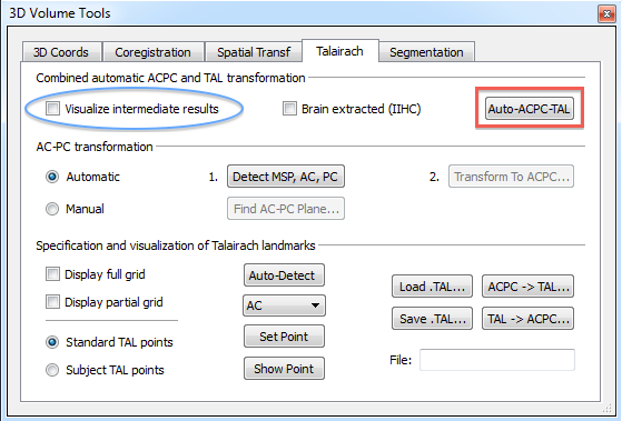
In order to run the automatic Talairach transformation, a click on the Auto-ACPC-TAL button (see above) in the Talairach tab of the 3D Volume Tools dialog is sufficient. The procedure may be started with a VMR data set that has just been created, i.e. without preprocessing such as inhomogenity correction and brain masking. It is, however, advised to first run the IIHC procedure. The Brain extracted (IIHC) check box will be on in case that the program finds evidence (by checking the name of the VMR file) that IIHC has been performed; this option will use slightly different parameters in sub-sequently applied tools. In case you do not use default names suggested by BrainVoyager, you may want to change the default setting of this option if needed.
After starting the automatic AC-PC and Talairach procedure, the program creates and loads both an AC-PC data set and a final Talairach data set from the original data set. It is recommended to turn on the Visualize intermediate results option since it visualizes several intermediate outcomes as a series of images in the Image Reporter (see below) that help to understand the performed steps and is also indicative of potential problems. Below each image a short text provides a description of the content in the image. Furthermore, additional information about fine-grained sub-steps is plotted in the Log pane during processing.
The automatic procedure performs a series of sub-steps. First, the mid-sagittal plane (MSP) is detected allowing to rotate the brain into sagittal orientation; as the sagittal center of the brain, the MSP contains the AC and PC connecting the left and right hemisphere (see snapshot of Image Reporter below).
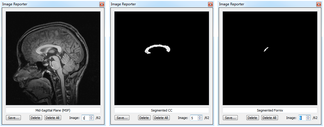
Then the corpus callosum (CC) is detected as a first reference for detecting the AC and PC point. The second snapshot above shows image no. 5 showing the successfully detected CC (see image above). Below the corpus callosum the Fornix is detected since the AC point is located below the inferior end of that structure (third snapshot, image no. 9).
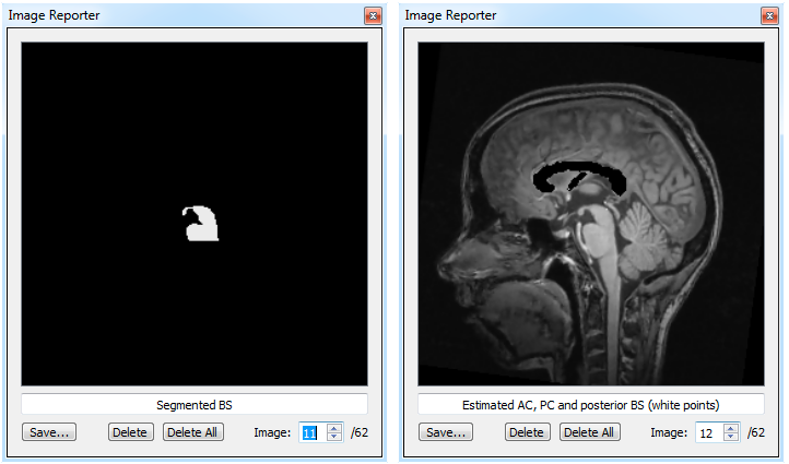
To detect the posterior commissure, the brain stem is segmented (see snapshots above, image no. 11) since the posterior commissure is superior to the dorsal posterior part of the brain stem. The initial AC and PC points are further refined by local search procedures ans shown as white dots in the Image Reporter (see snapshot above, image 12). The detected MSP, AC and PC points are then used to perform the AC-PC transformation step. The calculated transformation file (.trf) is stored to disk and the resulting ACPC VMR file is loaded. Note that the .trf and .vmr file names receive the trailing substring "_aACPC" indicating AC-PC space and that the result was obtained using the automatic ("a") procedure.
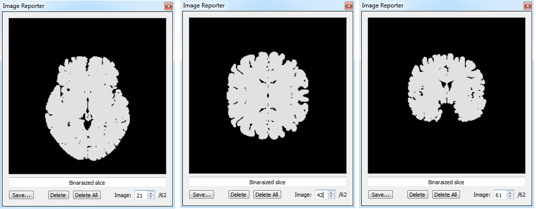
The automatic procedure then continues with the detection of the cerebrum border reference points using the loaded "[name]_aACPC.vmr" file as input. First the PC position is determined within the AC-PC plane. The cerebrum borders are then detected by segmenting the brain in several axial and coronal slices on which the most extreme borders of the calculated segments are determined. The comparison across slices is used to avoid outliers, i.e. slices where the segmentation did not work as desired; these slices may still contain non-brain tissues such as meninges that would lead to wrong cerebrum border estimations. The snapshots above shows 3 segmented slices where the segmentation works as desired, an axial slice (image no. 21), a mirrored half coronal slice (image no. 42) and a coronal slice (image no. 61). The final border points are estimated in the original aACPC data set with small adjustments that take into account intensity gradients and partial volume sampling. Finally the detected landmarks are saved in a "[name].tal" file and the Talairach normalization step is applied to the AC-PC VMR file resulting in an output file in Talairach space; the final VMR file uses the same name as for the AC-PC file but the "_aACPC" substring will be replaced with the "_aTAL" substring indicating that the resulting file is in Talairach space.
The automatic detection process works in a few seconds but the application of the ACPC and TAL transformation may take about a minute since it uses high-quality spatial interpolation schemes (cubic spline interpolation for ACPC transformation and sinc interpolation for the final TAL transformation). Although this provides perfect interpolation results, you may use the "reapply transformation" feature to run both steps (aACPC and aTAL) in a single transformation with the sinc interpolation option.
Verification of obtained results
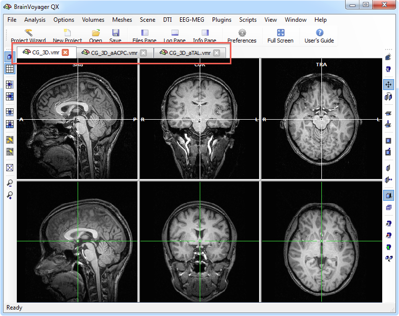
In many cases the automatic AC-PC and Talairach transformation steps work as expected. Since there may, however, be cases with erroneous results, it is strongly advised to check the obtained results. BrainVoyager tries to identify problems and issues warnings (e.g. that important anatomical structures like the corpus callosum or fornix could not be detected). The program makes it easy to verify the results by keeping 3 VMR files in the workspace: the original VMR, the AC-PC transformed VMR and the Talairach transformed VMR. You may switch between these 3 VMRs by clicking the respective tab bar buttons (see red rectangle in snapshot below). The original VMR is shown in two-row mode and can be used to check whether the cross in the lower row is indeed located at the AC point and that the PC point is located in the same axial slice (which is clearly the case in the example below). In case of non-ideal results, you may also inspect the images in the Image Reporter to localize potential problems. Note that you can easily correct the position of the AC point and (subsequently) the rotation angles for the PC point using the spin boxes in the Translation and Rotation fields of the Coregistration tab in the 3D Volume Tools dialog.
Copyright © 2014 Rainer Goebel. All rights reserved.