BrainVoyager QX v2.8
Applying SVMs to ROIs
Support vector machines are often applied to the responses of voxels in a regions-of-interest. Restricting the voxels to a ROI is conceptually interesting allowing to ask the question whether the response patterns in a specific brain region can be discriminated. Besides this conceptual point, such a "ROI-SVM" also helps to reduce the "curse of dimensionality" implementing one form of feature selection.
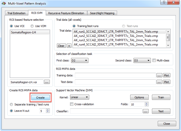
The ROI-SVM tab of the Multi-Voxel Pattern Analysis dialog (see snapshot above) allows to run SVMs on the data of a selected region-of-interest (ROI). The selected ROI can be as big as the whole cortex or as small as a few voxels.
Input 1 - Region-Of-Interest
In order to load a relevant volume-of-interest (VOI) file, use the "..." selection button in the ROI-based feature selection field. In the appearing list of VOIs, select the one you want to use for feature selection. In the example snapshot above, the VOI "SomatoRegion-LH" encompasses a region in the left hemisphere including somatosensory cortex since distributed responses in that part of the brain are of interest in this experiment.
Input 2 - Single-Trial Response Estimates
When the MVPA dialog has not been closed, the single-trial VMP files created in the Trial Estimation tab, appear directly in the Trial data field. Otherwise the desired VMP files can be added using the "+" selection button in the Trial data (all voxels) field (note that you can use multi-file selection).
Generation of Training and Test Patterns
The First class and Second class selection boxes in the Selection of classification task field can be used to specify which two conditions should be compared in case that trial estimates for more than two conditions are stored in the selected VMP files. In the example data, three conditions are used and one of the three possible pairs, "D2" and "D3" are selected. When using trials from these two conditions, a SVM will attempt to learn to classify the trials from these two conditions. It is also possible to set up training for multiple classes (e.g. all three classes in the example) by selecting the Multi-class option in the Selection of classification task field. With a selected VOI, a list of VMP files, and a specified classification task, the actual training data for the SVM classifier can be generated by clicking the Create button in the Create ROI-MVPA data field (see snapshot above).
Note that the executed ROI-MVPA data creation step will not only create training data but also data for testing the generalization performance of the trained classifier. There are two options for separating training and test data. If you have several experimental runs and you want to keep apart one (or more) runs for testing (recommended, if possible), switch to the Separate training / test runs option. Then you can fill the trial data list separately with training and test data. After clicking the Create button, only the data specified as training runs will be used to generate training patterns, while the data specified as test runs will be set apart for testing purposes. If you decide instead to use a proportion of the trial data from all runs for testing, select the Leave N out option in the Create ROI-MVPA data field and specify in the spin box on the right side of this option how many trials you want to randomly extract for testing the classifier. Note that the number entered here will be applied to each class. If the value is set to "5", 5 trial estimates will be picked out from each class and set aside for testing.
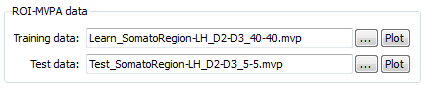
The snapshot above shows the ROI-MVPA data field of the ROI-SVM tab after clicking the Create button using the Leave N out option with N=5. The training and test data has been created and the corresponding output file names are shown. The name of the files describe what they contain, e.g. the "Learn_SomatorRegion-LH_D2-D3_40-40.mvp" file name indicates that this MVP file contains 40 patterns for class "D2" and 40 patterns for class "D3" and that the patterns are defined over the voxels (features) of the "SomatoRegion-LH" ROI. The name of the file containing the test patterns "Test_SomatoRegion-LH_D2-D3_5-5.mvp" indicates that it contains 5 patterns per class as requested with the Leave N out option. Note that the Log pane shows which patterns have been separated for the test patterns. In the example, the following lines are printed to the log:
No of all training data trials for class1, class2: 45  45
Class 1 trials removed for testing: 18 43 19 78 38
Class 2 trials removed for testing: 67 34 29 47 31
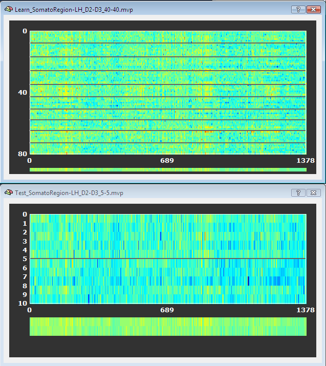
The format of the generated MVP files has been described in the Support Vector Machines section. Instead of two features used there, each pattern now contains about 1500 entries, which is the number of voxels in the specified "SomatorRegion-LH" ROI. The training and test patterns can be visualized by clicking the respective Plot buttons in the ROI-MVPA data field. Note that if one wants to run another classifier on the same data, one needs not to re-create the ROI trial data but one can directly select the desired MVP files (if already existing) using the "..." selection buttons. The plots below show the training and test data as stored in the MVP file. The separating lines indicate a switch between trials of class 1 and class 2. There are 9 lines for the training data since the trials from the different VMP files are appended to create the MVP file. On the bottom of the plot, the average response across all trials for class 1 (upper row) and class 2 (lower row) are shown.
SVM Model Selection
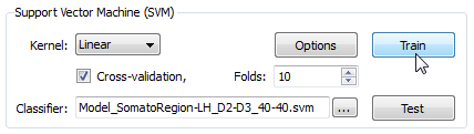
When the MVP data is created, a support vector machine can be trained. When the Train button is clicked in the Support Vector Machine (SVM) field, the data file listed in the Training data text field. This would use a SVM with default settings including a linear kernel and a value of "1" for the penalty parameter "C". While it is possible to select a non-linear kernel using the Kernel combo box in the Support Vector Machine (SVM) field, it is recommended to stick to the default linear kernel since this allows to use the weight vector of the trained SVM for visualization and feature selection.
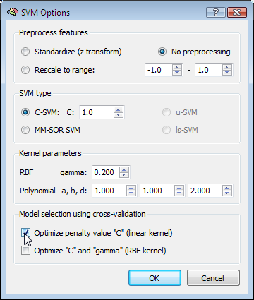
While using a linear kernel is appropriate, it is important to optimize the C parameter to create a classifier with good generalization performance (reflected by the size of the margin). A good model selection technique combines systematic parameter search with n-fold cross-validation. To enable this technique, invoke the SVM Options dialog by clicking the Options button in the Support Vector Machine (SVM) field. The first field in this dialog, Preprocess features, allows to standardize or rescale the data of a feature across the available patterns. This is important in case that the different features have very different variance, but it is normally not necessary when using z normalization during the trial estimation step. The SVM type field allows to set a desired value for the C parameter for SVM training. To let the program search for the optimal C parameter, the Optimize penalty value "C" (linear kernel) option can be checked in the Model selection using cross-validation field, which will systematically test values for C in a wide range.
SVM Training and Testing
After clicking the OK button, make sure that the Cross-validation option is also turned on in the Support Vector Machine (SVM) field of the Multi-Voxel Pattern Analysis dialog and set a value for the number of folds (or keep the default value "10"). To run the model selection process, click the Train button. Since we turned on parameter optimization with cross-validation, a series of SVMs with different C values will be generated and the test performance of each model will be evaluated using cross-validation. The Log pane will inform about the progress with the following output (only a subset of the printed lines are shown):
Testing parameter C=0.00673795 with 10-fold cross validation - Accuracy: 92.5%
Testing parameter C=0.011109 with 10-fold cross validation - Accuracy: 91.25%
:
Testing parameter C=1.64872 with 10-fold cross validation - Accuracy: 91.25%
Testing parameter C=2.71828 with 10-fold cross validation - Accuracy: 93.75%
Testing parameter C=4.48169 with 10-fold cross validation - Accuracy: 91.25%
:
Testing parameter C=1.2026e+06 with 10-fold cross validation - Accuracy: 88.75%
Testing parameter C=1.98276e+06 with 10-fold cross validation - Accuracy: 91.25%
Setting C to value resulting in best generalization performance: C=2.71828
Running SVM with C=2.71828 and linear kernel
After evaluating SVMs with different C parameter values, the program decides on using the value C=2.7, which produced the highest cross-validation accuracy (93.75% correct classification). Using the whole training data, it runs a final SVM training process with this C value. The performance on the training data is also plotted in the Log pane (only the prediction output of the last 20 of all 80 patterns is shown):
:
1.00036    1
1.23035    1
0.99963    1
1.00025    1
1.00006    1
0.999548   1
1.09946    1
1.16695    1
-1.00018  -1
-1.00031  -1
-0.999842 -1
-0.999998 -1
-1.19388  -1
-1.00022  -1
-1.04356  -1
-1.00034  -1
-0.9996   -1
Accuracy (full training set): 100%
The left column shows the predicted value and the right column the "label" indicating to which class the respective pattern actually belongs ("1" class 1, "-1" class 2). The trained SVM model is saved in a SVM file allowing to re-use the classifier in the future. The name of the stored SVM file is shown in the Classifier text box within the Support Vector Machine (SVM) field. In the snapshot above, the obtained SVM file is "Model_SomatoRegion-LH_D2-D3_40-40.svm"; the created file name is derived from the name of the used training data allowing to identify the MVP data belonging to the SVM model. The trained SVM can now be used to classify the test data, which was not used during model selection. When pressing the Test button, the data contained in the file shown in the Test data text box of the ROI-MVPA data field will be used as input for the trained SVM shown in the Classifier text box of the Support Vector Machine (SVM) field. After pressing the Test button, the predicted values fort the 10 test cases of our sample data are printed in the Log pane:
SVM output - predictions (plus targets) for test exemplars:
0.476441                      1
0.990862                      1
0.79285                       1
1.16716                       1
0.545607                      1
-0.618332                    -1
-0.299141                    -1
-0.557493                    -1
-0.0442947                   -1
-0.576111                    -1
Test data - prediction accuracy (assuming labels are known): 100%
This result shows that the classifier has indeed learned how to weight the voxels (features) of the ROI to discriminate between the two classes also for new test cases. While a performance of 100% is impressive, the results will be less good when less cases are used for learning and, hence, more cases are used for testing. In order to test, for example, the performance when setting 33% of the 45 trials per class for testing (instead of 11% or 5 cases), set a value of 15 in the Leave N out spin box and rerun the described steps. If accurracy values are not close to 100%, it is important to test whether obtained values are significant.
Visualizing the Weight Vector
The weights of a trained SVM together with the bias term define the discriminant functions of the classifier (see previous blog). In case of a linear classifier, the absolute value of a weight can be interpreted as the strength of contribution of the respective voxel to the multivariate classification. It is thus useful to visualize the weights of the involved voxels to obtain a "SVM map", which aids in making the "machine learning black box" more transparent.
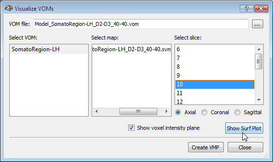
Visualizing the weights requires the knowledge which voxel (i.e. the respective x, y, z coordinates) corresponds to a specific weight. This link is lost when the MVP data file is created since this file only stores the estimated trial response values per voxel, but not the coordinates of a voxel. To keep that link alive, BrainVoyager actually saves a special "VOM" (volume-of-interest map) file to disk containing the coordinates of each ROI voxel. The link to the MVP data and SVM weight vector is kept alive since the VOM file lists the coordinates of voxels in the same order as used for weights in the MVP and SVM weight vector. While a VOM file is saved already during creation of the MVP data, the weight values are added after training the classifier. To visualize the weight vector of a SVM, use the Visualize VOMs dialog, which can be launched from the Options menu. The Browse button ("...") in the top part of the dialog allows to select the desired VOM file, which has the same name as the trained SVM except that the extension is changed from ".svm" to ".vom".
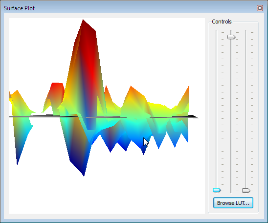
There are two different ways to visualize the weights over the corresponding voxels. One way presents the weights in a 3D plot for selected axial, coronal or sagittal slices (see snapshot above). This view allows to inspect in great detail how the weights are spatially distributed. You can drag the mouse within the plot to perform rotations or use the sliders on the right side. It is also possible to change the color look-up table by using the Browse LUT button.
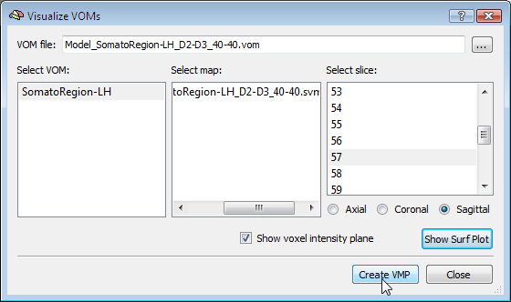
Another option to visualize the weights is in form of a standard volume map (see snapshot below). This can be achieved directly from the Visualize VOM dialog by clicking the Create VMP button (see snapshot above). Note that the map is in "native resolution", i.e. in the same resolution as the original VTC data and not in anatomical resolution (except if the VTC data has the same resolution). To ensure that the whole SVM analysis is based on native resolution data, the VOI used during the MVP data creation step is actually transferred from high-resolution (1 VOI voxel = 1 anatomical voxel) to the resolution of the VTC data. If the VTC data is represented in resolution "2" or "3", 1 functional voxel equals 2 x 2 x 2 / 3 x 3 x 3 anatomical voxels. Only after this transformation has been done, the trial estimates of the VTC data are linked to the VOM voxels keeping ROI voxel representations at native resolution.
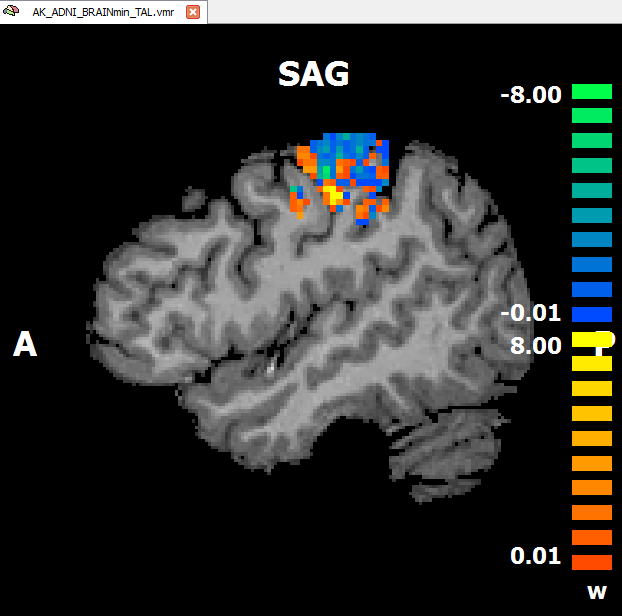
An advantage of visualizing the weight vector as a volume map is that it can be thresholded allowing to quickly check for the most relevant voxels by increasing the threshold. Since the weights may be very small when having several thousand features, the weight values are scaled when creating the newly introduced "w" (weight) map type (see snapshot above). The performed scaling process maps the values in the range from 0 to the maximum absolute value to a range from 0 to 10.
Support Vector Machines are not only useful for ROI-SVMs, but they play also an important role in the recursive feature selection tool allowing to find the most discriminative voxels within large brain regions.
Copyright © 2014 Rainer Goebel. All rights reserved.