BrainVoyager QX v2.8
Slice Scan Time Correction
An important step of preprocessing, especially for event-related designs, is the proper treatment of differences in the time when individual slices are recorded. The problem of different slice scanning times stems from the fact that a functional volume (e.g. whole brain) is usually not covered at once but with a series of successively measured 2D slices. For a functional volume of 30 slices and a volume TR of 3 seconds, for example, the data of the last slice is measured almost 3 seconds later than the data of the first slice. Despite the sluggishness of the hemodynamic response, an imprecise specification of time in the order of 3 seconds will lead to suboptimal statistical analysis, especially in event-related designs.
One way to cope with slice scanning time differences would be to shift the expected BOLD time course in time to compute proper statistical results. In this predictor-shifting approach, the reference time courses for a slice are shifted in time proportionally to the temporal difference in san time with respect to the reference (e.g. first) slice. Another possibility is to shift the data of a slice in time to the same time point as when the reference slice was scanned. This changes the data in a way as if the whole volume would have been measured at the same moment in time. Note that in the latter case, the same predictors can be used throughout the volume, i.e. slice-specific shifts of the precictors are no longer necessary. For this reason, the latter approach is normally used in fMRI data analysis, allowing to use the same predictors also after transforming the slice-based representation of the functional data (FMR/STC)to a 3D representation of the data (VTC) in an arbitrary (e.g. AC-PC or Talairach) space. It also allows to compare and integrate event-related responses from different brain regions correctly with respect to temporal parameters such as onset latency. The predictor-shifting approach would require that each voxel would keep a label indicating the slice from which it originates so that the correct shifted set of predictors could be used. Note that the data-shifting approach requires interpolation (resampling) of the slice time courses (see below).
Slice Scanning Order
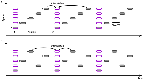
In order to correct for different slice scan timings, the time series of individual slices are "shifted" in time to match a reference time point, e.g. the first or middle slice of a functional volume. This temporal shift depends on the order in which the individual slices of a volume are scanned. Besides an ascending or descending order, slices are often scanned interleaved, i.e. the odd slice numbers are recorded first followed by the even slice numbers. The figure above shows an example of ascending scanning (top) and interleaved scanning order (bottom) for five slices. The time points of original scan times are indicated with gray rounded rectangles, while the shifted data are depicted with pink rectangles. The resampled data can be treated as if all slices of one functional volume would have been scanned at the same time point. Note that in case that the header of the original data contains slice timing information, this data is used (since version 2.8.2) because it is assumed that header information is the most accurate one (see below).
Temporal Interpolation
As described above, correcting differences in slice timing using the data-shifting approach requires to re-sample the data at time points falling in-between measured data points. The values at the non-measured time points can be estimated by using measured data points "in the neighborhood" i.e. from time points measured in close proximity. In BrainVoyager QX, three interpolation methods are available, linear, cubic spline and windowed sinc interpolation. The linear interpolation method uses only the neighbor on the left and on the right side to calculate the value at the resampled point. It implements an average of these values weighted by the relative distance: xtnew = (1-Δ)*xt-1 * Δ*xt. The linear interpolation method is fast to compute but has the disadvantage that it smoothes the data. Furthermore, the introduced smoothing depends on the slice, i.e. it is negligible if points are resampled close to a measured point but smoothing is rather strong if points are resampled in the middle between two measured points (see below). The two other interpolation schemes, cubic spline and since interpolation, avoid this problem by using more points in the neighborhood leading to a very accurate resampling.
In the following, the different interpolation methods are compared using the first 50 volumes of the "Objects" sample data set (the first two volumes have been skipped, i.e. volumes 3 - 52 are used from the original data). The sample data consists of 25 slices, which are scanned within 2 seconds (TR) in an interleaved ascending order.
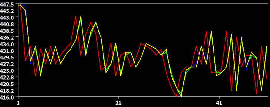
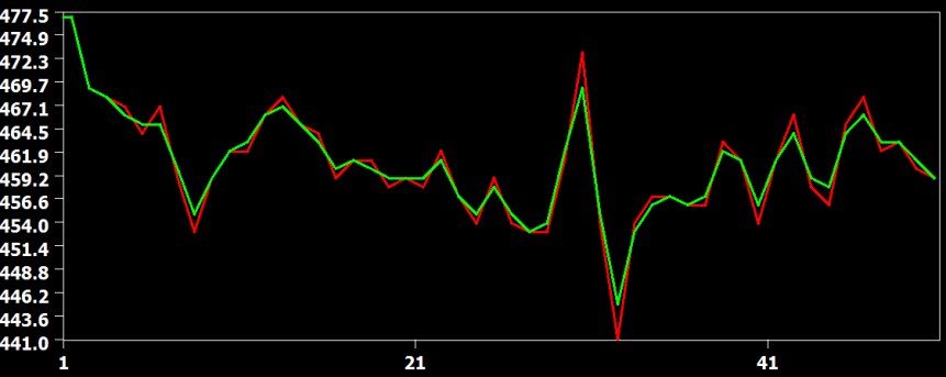
The figure above shows the original time course of a voxel in red from slice 22, which is the slice before the last slice scanned within a volume. In this case, the data has to be shifted forward almost for one full TR and the figure shows that all interpolation methods are performing this shift very well without significant deviations from each other. The curve from the linear interpolation method is shown in green, the cubic spline method in blue and the sinc method in yellow. Since the sinc curve is plotted last, the linear and cubic spline curve are hidden behind due to the similarity in the interpolation result.
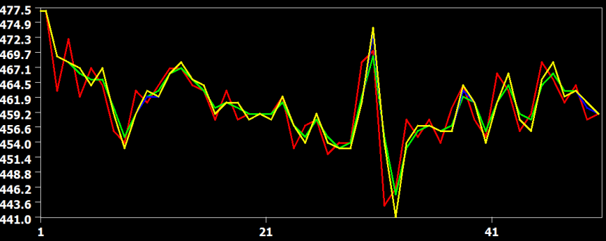
In the figure above the raw data (red) and the result from the three interpolation methods are shown for slice 23, which is the slice scanned prior to the middle slice. In this situation, the time course must be shifted about half a TR, i.e. time points must be "recreated" in the middle between two measured time points. In this situation, the cubic spline (blue) and sinc (yellow) interpolation method are performing very similar but the linear interpolation method introduces visible smoothing. This is shown in more detail in the two subsequent figures.
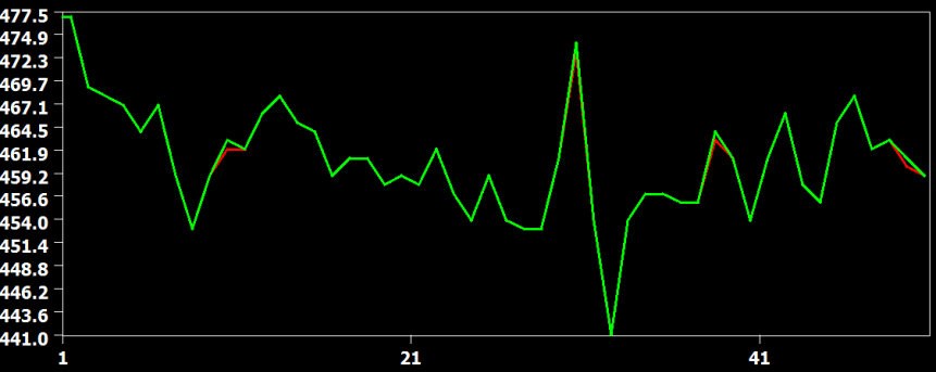
The figure above compares the cubic spline (red) and sinc (green) interpolation method, showing that they produce identical results (the green curve hides the red curve). The figure below compares the interpolation result from the cubic spline (red) and the linear (green) interpolation method. Here it becomes clear that the linear interpolation method smoothes the data as is apparent in weaker up and down deflections in the green as compared to the red curve.
The examples confirm the theoretically expected behavior of the interpolation methods demonstrating slice-dependent smoothing of the linear method. Therefore cubic spline or windowed sinc interpolation should be used for slice scan time correction. Cubic spline interpolation is set as the default method in the FMR Data Preprocessing dialog (see screenshot below from the right upper part of the dialog).
Slice Time Tables and Multiband Scans
In recent years, parallel excitation techniques are gaining increasing interest that work by exciting more than once slice in parallel: If, for example, 8 slices are excited simultaneously, a whole-brain scan with 64 slices would be completed in the same time as 8 non-simultaneously recorded slices. In order to enable such powerful “multiband” techniques, advanced excitation hardware (multiple transmit channels) and special MRI pulse sequences are needed. Since multiple slices are acquired truly in parallel, imaging time is substantially reduced as compared to standard single-slice excitation techniques. Note that the usual slice scanning order settings arrange all slices in a specific scanning sequence. In order to handle multiband acceleration, a new option has been added in the Slice Scanning Order dialog (see below) allowing to specify the multiband acceleration factor in the Multiband field.
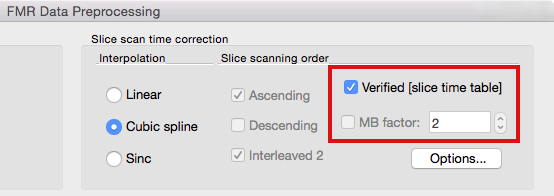
Since setting (multiband) slice timing manually might become challenging, BrainVoyager (since version 2.8.2) attempts to set scanning order automatically based on detailed slice-specific timing data in case it is available in the header of the original image files. If available, slice timing data is extracted from the first volume (and eventually second volume for cross-checking) and stored in created .FMR project files. This data is referred to as a slice time table because it indicates for each slice when it has been recorded relative to acquisition onset of the respective volume. Since it is stored in the FMR file, the slice time table is then available when preprocessing the functional data. At present, slice timing data is extracted from SIEMENS mosaic DICOM files (from the so-called CSA header). If this data is available, the Verified [slice time table] option appears in the FMR Data Preprocessing dialog (see below). This option is then turned on as default and overrules the usual slice scanning order settings that are disabled (greyed out, see below); while not recommended, it is possible to turn this option off and to use conventional slice order settings.
The slice time table is also visible in the Slice Scanning Order dialog: the timing value printed below each slice (see below) is the value extracted from the header and not calculated as in the conventional case from the TR and inter slice timing values.
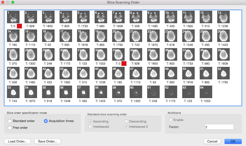
The screenshot above shows that the Acquisition time option is automatically turned on in the Slice order specification mode field in case that the slice time table is available. Note that the Standard slice scanning order and Multiband fields are disabled since all necessary information is directly used from the slice time table. Value "2" in the Factor spin box of the Multiband field indicates that in this data a multiband sequence with acceleration factor 2 has been detected. The red square in the snapshot indicates the begin of the first and second "band", i.e. it is the first pair of slices that is recorded simultaneously at time point 0. Note that in case of an available slice time table, no settings have to be changed in this dialog.
Copyright © 2014 Rainer Goebel. All rights reserved.