BrainVoyager QX v2.8
Fixed Effects, Random Effects, Mixed Effects
After (Talairach or cortex-based) brain normalization, the whole-brain/cortex data from multiple subjects can be statistically analyzed simply by concatenating time courses at corresponding locations. After concatenation, the same statistical analysis as described for single subject data can be applied. In fact, in the context of the GLM, the multi-subject voxel time courses as well as the multi-subject predictors may be obtained by appending the data and design matrices of all subjects. After estimating the beta values, contrasts can be tested in the same way as described for single subject data.
Fixed-Effects Analysis
The concatenation approach leads to a high statistical power since a large number of events are used to estimate the beta values, i.e. the number of analyzed data points is the sum of the data points from all subjects; in case that all N subjects have the same number of data points n, the total number of data points NT is NT = N x n. Note, however, that the obtained statistical results (e.g. contrast t maps) from concatenated data and design matrices cannot be generalized to the population level since the data is analyzed as if it originates from a single subject that is scanned for a (very) long time. Inferences drawn from obtained results are only valid for the included group of subjects since the group data is treated like a virtual single-case study. In order to test whether the obtained results are valid at the population level, the statistical procedure needs to consider that subjects constitute a randomly drawn sample from a large population. Subjects are thus random quantities and the statistical analysis must assess the variability of observed effects between subjects (![]() ) in a random effects (RFX) analysis. In contrast, the simple concatenation approach constitutes a fixed effects (FFX) analysis assessing observed activation effects with respect to the scan-to-scan measurement error, i.e. with respect to the precision with which we can measure the fMRI signal. The source of variability used in a FFX analysis, thus, represents within-subject variance (
) in a random effects (RFX) analysis. In contrast, the simple concatenation approach constitutes a fixed effects (FFX) analysis assessing observed activation effects with respect to the scan-to-scan measurement error, i.e. with respect to the precision with which we can measure the fMRI signal. The source of variability used in a FFX analysis, thus, represents within-subject variance (![]() ).
).
Random-Effects Analysis
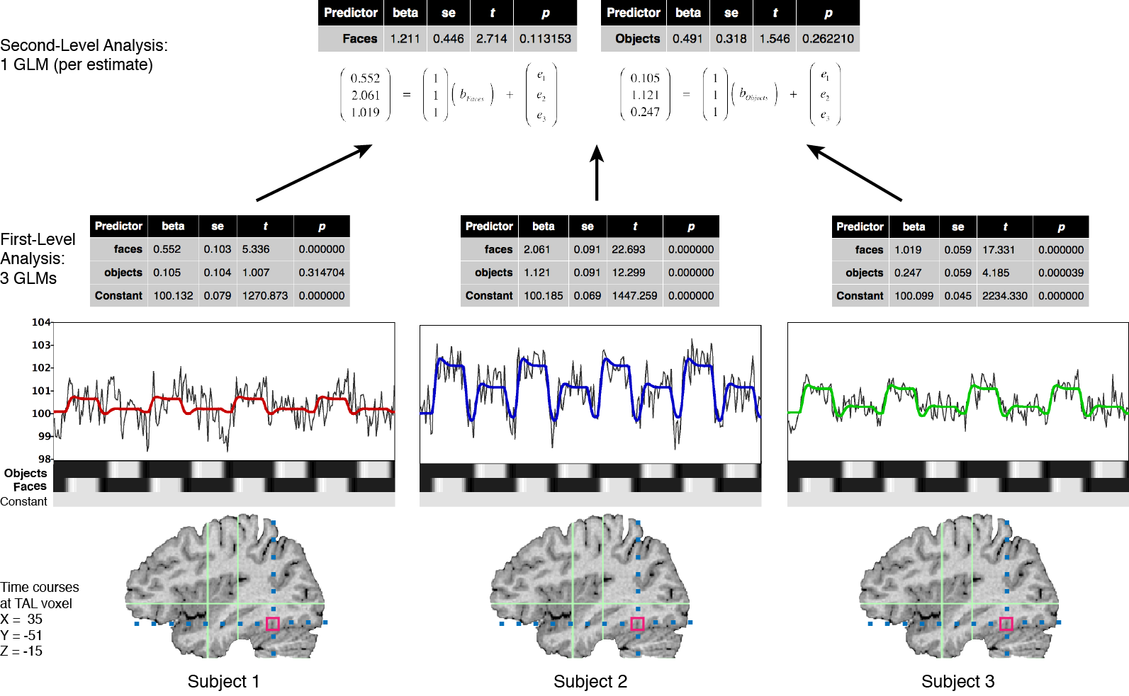
The optimal approach to perform valid population inferences is to run a single GLM using the full time course data from all subjects as in the simple concatenation approach described above. Instead of simple concatenation, however, a special multi-subject design matrix is created that allows modeling explicitly both within-subjects and between-subjects variance components (ref; Beckmann et al., 2003). Because this “all-in-one” approach leads to large concatenated data sets and huge design matrices that are difficult to handle on standard computer platforms, many authors have proposed to separate the group analysis in (at least) two successive stages by performing a multi-level analysis (e.g. Holmes and Friston, 1998; Worsley et al., 2002; Beckman et al., 2003; Woolrich et al., 2004; Friston et al., 2005). The suggested analysis strategies are related to the multi-level summary statistics approach (e.g. Kirby, 1993). In the first analysis stage, parameters (summary statistics) are estimated for each subject independently (level 1, fixed effects). Instead of the full time courses, only the resulting first-level parameter estimates (betas or contrast of betas) from each subject are carried forward to the second analysis stage where they serve as the dependent variables. The second level analysis assesses the consistency of effects within or between groups based on the variability of the first-level estimates across subjects (level 2, random effects). This hierarchical analysis approach reduces the data for the second stage analysis enormously since the time course data of each subject has been “collapsed” to only one or a few parameter estimates per subject. Since the summarized data at the second level reflects the variability of the estimated parameters across subjects, obtained significant results can be generalized to the population from which the subjects were drawn as a random sample.
To summarize the data at the first level, standard linear modeling (GLM) is used to estimate parameters (beta values) separately for each subject k.
[fig]
Instead of one set of beta values as in the concatenation approach, this step will provide a separate set of beta values bk for each subject. The obtained beta values serve as the dependent variable at the second level and can be analyzed again with a general linear model:
[fig]
Note that the error term eG is a random variable that specifies the deviation of individual subjects from group parameter estimates, i.e. it models the random-effects variability (actually a combination of within-subject and between-subject variance, see below). The group design matrix XG may be used to model group mean effects of first-level beta estimates of a single condition or contrast values (one per subject), implementing e.g. a one-sample t-test with a simple design matrix containing just a constant (“1”) predictor (see fig. x). More generally, any mixed design with one or more within-subjects factors and one or more between-subjects factor can be analyzed using a GLM / ANOVA formulation at the second level.
Mixed-Effects Analysis
The random-effects analysis at the second level described above does not differ from the usual statistical approach in behavioral and medical sciences: The units of observation are measurements from randomly and independently drawn subjects with (usually) fixed experimental group factors (e.g. specific patient groups as levels), fixed repeated measures factors (e.g. specific tasks as levels) and one or more covariates (e.g. age or IQ). We know, however, from the first level analysis that our “measurements” are parameter estimates and not the true (unobservable) population values. With parameter estimates as the dependent variable (instead of error-free true values), the second level can no longer be treated as a pure random-effects model since the entered values are “contaminated” by variance from the first level analysis. The second level, thus, becomes a mixed-effects (MFX) model containing variance components from both the first (fixed effects) and second (random effects) level. It can be shown (see also below) that the two-level summary statistics approach nonetheless leads to valid inferences but it requires that the variances of first-level parameter estimates are homogeneous across subjects. A safe way to correctly estimate the fixed and random effects variance components is to avoid the summary statistics approach and to construct the “all-in-one” model mentioned earlier that combines the two levels in one equation:
[fig]
The resulting well-known mixed-effects model (Verbeke and Molenberghs, 2000) can be fitted using e.g. the generalized least squares (GLS) approach (see section x). This model does not use the summary statistics approach since the group betas are directly estimated from the full time series data of all subjects. The resulting betas bG are used to test contrasts at the group level with standard deviation values that take into account (inhomogeneous) fixed and random effects variance components This approach leads to large design matrices and data sets and is challenging to perform on standard computer platforms but it leads to valid inferences even in case of unbalanced designs (see below).
It would, thus, be advantageous to use the multi-level summary statistics approach described above to perform mixed-effects analysis. Since the first-level betas are only estimates of the true (population) betas, the two-level model is, however, not strictly identical to the all-in-one model. Nonetheless it has been shown that by incorporating first-level information about the precision (variance) of the estimated betas (as well as their covariance) into the second level model, a two-level summary statistics approach may be performed that is identical to the all-in-one model (Beckmann et al., 2003; Friston et al., 2005). Since in this case both first-level and second-level variance components are incorporated at the second level, the analysis extends a random-effects model to a mixed-effects model allowing for non-homogenous variances at the first level. Solutions of these modified two-stage mixed effects models require, however, time-consuming iterative estimation procedures using frequentist (e.g. Worsley et al. 2002) or Bayesian (e.g. Woolrich et al., 2004; Friston et al., 2005) framework. A major advantage of mixed-effects (generalized two-level or all-in-one) models as compared to the simple two-level summary statistics model is that they can take into account different subject-specific first-level parameter variances. If, for example, a subject has a very high first-level beta value but it enters the second level also with a very high parameter variance, the mixed-effects model is able to “down-weight” its effect on the group variance estimates resulting in an effective treatment of outliers.
Balanced Designs
While the modified mixed-effects model do not require the homogeneous variance assumption, the simpler multi-level summary statistics approach (using non-iterative ordinary least squares (OLS) estimation) has been shown to be robust with respect to modest violations of the homogeneity-of-variance assumption (Fristion et al., 2005; Mumford & Nichols, 2009). More specifically, when calculating one-sample t-test contrasts of first-level parameter estimates, group inferences based on OLS estimation are fully valid and even achieve nearly optimal sensitivity under modest violations of the variance homogeneity assumption (Penny; Mumford & Nichols, 2009). For realistic scenarios, the power differences between advanced mixed-effects models and the simple two-stage summary statistics approach are modest (Penny; Friston et al., 2005; but see Beckmann et al., 2003). As a general advice, balanced designs should be employed whenever possible since such designs lead to valid estimates and inferences without complex iterative fitting routines.
If one considers how the variance of parameter estimates/contrasts are calculated, it becomes clear that it is a function of two major components, the design matrix and the variance of the residuals (Var(e)):
For simplicity, let’s consider the case that the contrast vector contains just one “1” entry and zeros otherwise, i.e. we consider the standard error of a single beta estimate bj of a predictor of interest pj. In that case the c’(X’X)-1c term will simply retrieve the diagonal element of the inverted X’X matrix. Assuming (largely) non-overlapping epochs for included main condition predictors, the extracted value will be close to 1/nj, i.e. it reflects the number of data points used to measure the respective condition of interest; the value will not be exactly nj since we usually do not use a boxcar predictor to specify stimulus events/blocks but predictors that are the result of convolution of the boxcar with a hemodynamic response function (see section x); under slightly simplified considerations, we obtain:
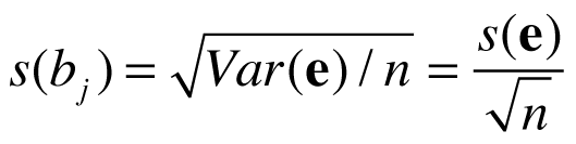
which is the usual equation to calculate standard errors, i.e. the standard deviation reduces with the square root of the number of observations (data points). If, for example, subject 1 uses 4x as many data points for condition j than subject 2, the standard error of the beta value of subject 1 will be sqrt(4) = 2 times smaller than the standard error of subject 2 (assuming equal s(e) values). To ensure a balanced design for group-level analysis, the respective condition should thus, be measured in each subject with the same amount of data points [footnote: this does not impose any restriction on the order of condition events/blocks within subject]; different conditions may have a different number of data points as long as the same number of data points is used for each subject.
The second term influencing the standard error of the estimated beta values is the (estimated) measurement error s(e). When using raw fMRI data, this value may differ substantially between subjects at corresponding voxels due to physical and physiological aspects of MRI scanning. It can be made more similar by adequate time course transformations, including percent signal change and baseline z-normalization. Consider subject 1 with a mean baseline value of 2000 and a mean value in condition j of 2050, and subject 2 with a mean baseline value at the same voxel of 1000 and a mean condition value of 1030. While subject 1 has a greater absolute effect (50) than subject 2 (30) the percent change is actually smaller in subject 1 (2.5%) than in subject 2 (3%). Since the fMRI signal changes are believed to scale with the level of the measured signal, a percent signal change (psc) transformation of each value with respect to the voxel time course mean value is usually performed before (group-level) statistical analysis: psc = yi / mean(y) *100. With this transformation, the mean value of the time course at a corresponding voxel will be the same (100) for all subjects and values of the time course are expressed as percent changes around that mean. This voxel-wise transformation should also make the error variance var(e) more similar at corresponding voxels across subjects since it is also assumed that the signal variance scales with the level of the measured raw signal.
Since the signal variance during baseline measurement points is an estimate of the error variance, a baseline z transformation (z=(y2-mean(y2))/s(y2) with y2 indicating baseline measurements) would ensure more stringently that different subjects have the same error variance. With this transformation, the strength of parameter estimates of subjects are expressed not as percent change but as units of standard deviation with respect to a subject’s error variance. While obvious, it needs to be stressed that each subject’s data should be preprocessed (see section x) in the same way in order to ensure as homogeneous within-subject variability as possible.
In summary, standard time course normalization combined with balanced designs lead to rather homogeneous standard errors of beta/contrast estimates across subjects and the two-level summary statistics approach, thus, leads to (near) optimal statistical results. Since the two-level summary statistics approach is robust with respect to modest violations of the homogeneous variance assumption (e.g. Mumford & Holmes), it’s application has become common practice (Friston et al., 2005). For designs deviating substantially from the equality of variance assumption (e.g. in designs requiring post-hoc classification of events), one of the more complex mixed effects analysis approaches should be employed.
Copyright © 2014 Rainer Goebel. All rights reserved.