BrainVoyager QX v2.8
The General Linear Model (GLM)
The described t test for assessing the difference of two mean values is a special case of an analysis of a qualitative (categorical) independent variable. A qualitative variable is defined by discrete levels, e.g., "stimulus off" vs. "stimulus on". If a design contains more than two levels assigned to a single or multiple factors, an analysis of variance (ANOVA) can be performed, which can be considered as an extension of the t test. The described correlation coefficient on the other hand is suited for the analysis of quantitative independent variables. A quantitative variable may be defined by any gradual time course. If more than one reference time course has to be considered, multiple regression analysis can be performed, which can be considered as an extension of the simple linear correlation analysis.
The General Linear Model (GLM) is mathematically identical to a multiple regression analysis but stresses its suitability for both multiple qualitative and multiple quantitative variables. The GLM is suited to implement any parametric statistical test with one dependent variable, including any factorial ANOVA design as well as designs with a mixture of qualitative and quantitative variables (covariance analysis, ANCOVA). Because of its flexibility to incorporate multiple quantitative and qualitative independent variables, the GLM has become the core tool for fMRI data analysis after its introduction into the neuroimaging community by Friston and colleagues (Friston et al. 1994, 1995). The following sections briefly describe the mathematical background of the GLM in the context of fMRI data analysis; a comprehensive treatment of the GLM can be found in the standard statistical literature, e.g. Draper and Smith (1998) and Kutner et al. (2005).
Note: In the fMRI literature, the term "General Linear Model" refers to its univariate version. The term "univariate" does in this context not refer to the number of independent variables, but to the number of dependent variables. As mentioned earlier, a separate statistical analysis is performed for each voxel time series (dependent variable). In its general form, the General Linear Model has been defined for multiple dependent variables, i.e. it encompasses tests as general as multivariate covariance analysis (MANCOVA).
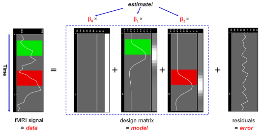
From the perspective of multiple regression analysis, the GLM aims to "explain" or "predict" the variation of a dependent variable in terms of a linear combination (weighted sum) of several reference functions. The dependent variable corresponds to the observed fMRI time course of a voxel and the reference functions correspond to time courses of expected (idealized) fMRI responses for different conditions of the experimental paradigm. The reference functions are also called predictors, regressors, explanatory variables, covariates or basis functions. A set of specified predictors forms the design matrix, also called the model. A predictor time course is typically obtained by convolution of a condition box-car time course with a standard hemodynamic response function (two-gamma HRF or single-gamma HRF). A condition box-car time course may be defined by setting values to 1 at time points at which the modeled condition is defined ("on") and 0 at all other time points. Each predictor time course X gets an associated coefficient or beta weight b, quantifying its potential contribution in explaining the voxel time course y. The voxel time course y is modeled as the sum of the defined predictors, each multiplied with the associated beta weight b. Since this linear combination will not perfectly explain the data due to noise fluctuations, an error value e is added to the GLM system of equations with n data points and p predictors:
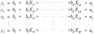
The y variable on the left side corresponds to the data, i.e. the measured time course of a single voxel. Time runs from top to bottom, i.e. y1 is the measured value at time point 1, y2 the measured value at time point 2 and so on. The voxel time course (left column) is "explained" by the terms on the right side of the equation. The first column on the right side corresponds to the first beta weight b0. The corresponding predictor time course X0 has a value of 1 for each time point and is, thus, also called "constant". Since multiplication with 1 does not alter the value of b0, this predictor time course (X0) does not explicitly appear in the equation. After estimation (see below), the value of b0 typically represents the signal level of the baseline condition and is also called intercept. While its absolute value is not informative, it is important to include the constant predictor in a design matrix since it allows the other predictors to model small condition-related fluctuations as increases or decreases relative to the baseline signal level. The other predictors on the right side model the expected time courses of different conditions. For multi-factorial designs, predictors may be defined coding combinations of condition levels in order to estimate main and interaction effects. The beta weight of a condition predictor quantifies the contribution of its time course in explaining the voxel time course. While the exact interpretation of beta values depends on the details of the design matrix, a large positive (negative) beta weight typically indicates that the voxel exhibits strong activation (deactivation) during the modeled experimental condition relative to baseline. All beta values together characterize a voxels "preference" for one or more experimental conditions. The last column in the system of equations contains error values, also called residuals, prediction errors or noise. These error values quantify the deviation of the measured voxel time course from the predicted time course, the linear combination of predictors.
The GLM system of equations may be expressed elegantly using matrix notation. For this purpose, we represent the voxel time course, the beta values and the residuals as vectors, and the set of predictors as a matrix:
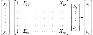
Representing the indicated vectors and matrix with single letters, we obtain this simple form of the GLM system of equations:

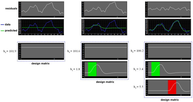
In this notation, the matrix X represents the design matrix containing the predictor time courses as column vectors. The beta values now appear in a separate vector b. The term Xb indicates matrix-vector multiplication. The figure above shows a graphical representation of the GLM. Time courses of the signal, predictors and residuals have been arranged in column form with time running from top to bottom as in the system of equations.
Given the data y and the design matrix X, the GLM fitting procedure has to find a set of beta values explaining the data as good as possible. The time course values predicted by the model are obtained by the linear combination of the predictors:

A good fit would be achieved with beta values leading to predicted values which are as close as possible to the measured values y. By rearranging the system of equations, it is evident that a good prediction of the data implies small error values:

An intuitive idea would be to find those beta values minimizing the sum of error values. Since the error values contain both positive and negative values (and because of additional statistical considerations), the GLM procedure does not estimate beta values minimizing the sum of error values, but finds those beta values minimizing the sum of squared error values:

The term e'e is the vector notation for the sum of squares (Sigma e2). The apostrophe symbol denotes transposition of a vector or matrix. The optimal beta weights minimizing the squared error values (the "least squares estimates") are obtained non-iteratively by the following equation:

The term in brackets contains a matrix-matrix multiplication of the transposed, X', and non-transposed, X, design matrix. This term results in a square matrix with a number of rows and columns corresponding to the number of predictors. Each cell of the X'X matrix contains the scalar product of two predictor vectors. The scalar product is obtained by summing all products of corresponding entries of two vectors corresponding to the calculation of covariance. This X'X matrix, thus, corresponds to the predictor variance-covariance matrix. The variance-covariance matrix is inverted as denoted by the "-1" symbol. The resulting matrix (X'X)-1 plays an essential role not only for the calculation of beta values but also for testing the significance of contrasts (see below). The remaining term on the right side, X'y, evaluates to a vector containing as many elements as predictors. Each element of this vector is the scalar product (covariance) of a predictor time course with the observed voxel time course.
An interesting property of the least squares estimation method is that the variance of the measured time course can be decomposed into the sum of the variance of the predicted values (model-related variance) and the variance of the residuals:
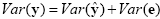
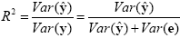
Since the variance of the voxel time course is fixed, minimizing the error variance by least squares corresponds to maximizing the variance of the values explained by the model. The square of the multiple correlation coefficient R provides a measure of the proportion of the variance of the data which can be explained by the model:
The values of the multiple correlation coefficient vary between 0 (no variance explained) to 1 (all variance explained by the model). A coefficient of R = 0.7, for example, corresponds to an explained variance of 49% (0.7x0.7). An alternative way to calculate the multiple correlation coefficient consists in computing a standard correlation coefficient between the predicted values and the observed values: R = ryy. This equation offers another view on the meaning of the multiple correlation coefficient quantifying the interrelationship (correlation) of the combined set of predictor variables with the observed time course.
GLM Diagnostics
Note that if the design matrix (model) does not contain all relevant predictors, condition-related increases or decreases in the voxel time course will be explained by the error values instead of the model. It is, therefore, important that the design matrix is constructed with all expected effects, which may also include reference functions not related to experimental conditions, for example, estimated motion parameters or drift predictors if not removed during preprocessing. In case that all expected effects are properly modeled, the residuals should reflect only noise fluctuations. If some effects are not (correctly) modeled, a plot of the residuals will show low frequency fluctuations instead of a stationary noisy time course. A visualization of the residuals is, thus, a good diagnostic to assess whether the design matrix has been defined properly.
GLM Significance Tests
The multiple correlation coefficient is an important measure of the "goodness of fit" of a GLM. In order to test whether a specified model significantly explains variance in a voxel time course, the R value can be transformed in an F statistic with p - 1 degrees of freedom in the numerator and n - p degrees of freedom in the denominator:
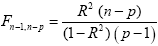
With the known degrees of freedom, an F test can be converted in an error probability value p. A high F value (low p value) indicates that one or more experimental conditions substantially modulate the data time course.
While the overall F statistic may tell us whether the specified model significantly explains a voxel's time course, it does not allow to asses which individual conditions differ significantly from each other. Comparisons between conditions can be formulated as contrasts, which are linear combinations of beta values corresponding to null hypotheses. To test, for example, whether activation in a single condition i deviates significantly from baseline, the null hypothesis would be H0: b1 = 0. To test whether activation in condition 1 is significantly different from activation in condition 2, the null hypothesis would state that the beta values of the two conditions would not differ, H0: b1 = b2 or H0: (+1)b1 + (-1)b2 = 0. To test whether the mean of condition 1 and condition 2 differs from condition 3, the following contrast could be specified: H0: (b1 + b2)/2 = b3 or H0: (+1)b1 + (+1)b2 + (-2)b3 = 0. The values used to multiply the respective beta values are often written as a contrast vector c. In the latter example , the contrast vector would be written as c = [+1 +1 -2]. Note that the constant term is treated as a confound and it is not included in contrast vectors, i.e. it is implicitly assumed that b0 is multiplied by 0 in all contrasts. To include the constant explicitly, each contrast vector must be expanded by one entry at the beginning or end. Using matrix notation, the linear combination defining a contrast can be written as the scalar product of contrast vector c and beta vector b. The null hypothesis can then be simply described as c'b = 0. For any number of predictors k, such a contrast can be tested with the following t statistic with n - p degrees of freedom:
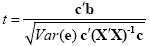
The numerator of this equation contains the described scalar product of the contrast and beta vector. The denominator defines the standard error of c'b, i.e. the variability of the estimate due to noise fluctuations. The standard error depends on the variance of the residuals Var(e) as well as on the design matrix X but not on the data time course y. With the known degrees of freedom, a t value for a specific contrast can be converted in an error probability value p using the equation shown earlier. Note that the null hypotheses above were formulated as c'b = 0 implying a two-sided alternative hypothesis, i.e. Ha: c'b != 0. A two-sided test is used as default in BrainVoyager QX. For one-sided alternative hypotheses, e.g., Ha: b1 > b2, the obtained p value from a two-sided test can be simply divided by 2 to get the p value for the one-sided test. If this p value is smaller than 0.05 and if the t value is positive, the alternative hypothesis may be concluded.
Conjunction Analysis
Experimental research questions often lead to specific hypotheses, which can best be tested by the conjunction of two or more contrasts. As an example, it might be interesting to test with contrast c1 whether condition 2 leads to significantly higher activity than condition 1 and with contrast c2 whether condition 3 leads to significantly higher activity than condition 2. This question could be tested with the following conjunction contrast:
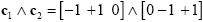
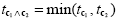
Note that a logical "and" operation is defined for Boolean values (true / false) but that t values associated with individual contrasts can assume any real value. An appropriate way to implement a logical "and" operation for conjunctions of contrasts with continuous statistical values is to use a minimum operation, i.e. the significance level of the conjunction contrast is set identical to the significance level of the contrast with the smallest t value:
Multicollinear Design Matrices
Multicollinearity exists when predictors of the design matrix are highly intercorrelated. To assess multicollinearity, pairwise correlations between predictors are not sufficient. A better way to detect multicollinearity is to regress each predictor variable on all the other predictor variable and examine the resulting R2 values. Perfect or total multicollinearity occurs when a predictor of the design matrix is a linear function of one or more other predictors, i.e. when predictors are linearly dependent on each other. While in this case solutions for the GLM system of equations still exist, there is no unique solution for the beta values. From a mathematical perspective of the GLM, the square matrix X'X becomes singular, i.e. it looses (at least) one dimension, and is no longer invertible in case that X exhibits perfect multicollinearity. Matrix inversion is required to calculate the essential term (X'X)-1 used for computing beta values and standard error values (see above). Fortunately, special methods, including singular value decomposition (SVD), allow obtaining (pseudo-) inverses for singular (rank deficient) matrices. Note, however, that in this case the absolute values of beta weights are not interpretable and statistical hypothesis tests must meet special restrictions. In fMRI design matrices, multicollinearity occurs if all conditions are modeled as predictors in the design matrix including the baseline (rest, control) condition. Without the baseline condition, multicollinearity is avoided and beta weights are obtained which are easily interpretable. As an example consider the case of two main conditions and a rest condition. If we would not include the rest condition (recommended), the design matrix would not be multicollinear and the two beta weights b1 and b2 would be interpretable as increase or decrease of activity relative to the baseline signal level modeled by the constant term (see figure above, right column). This approach is recommended in BrainVoyager and is especially important when running GLMs for random-effects group analyses. Contrasts could be specified to test single beta weights, e.g. the contrast c = [1 0] would test whether condition 1 leads to significant (de)activation relative to baseline. Furthermore, the two main conditions could be compared with the contrast c =[-1 1], which would test whether condition 2 leads to significantly more activation than condition 1. If we would create the design matrix including a predictor for the rest condition, we would obtain perfect multicollinearity and the matrix X'X would be singular. Using a pseudo-inverse or SVD approach, we would obtain now three beta values (plus the constant), one for the rest condition, one for main condition 1 and one for main condition 2. While the values of beta weights might not be interpretable, correct inferences of contrasts can be obtained if an additional restriction is met, typically that the sum of the contrast coefficients equals 0. To test whether main condition 1 differs significantly from the rest condition, the contrast c = [-1 +1 0] would now be used. The contrast c = [0 -1 +1] would be used to test whether condition 2 leads to more activation than condition 1.
GLM Assumptions
Given a correct model, the estimation routine (ordinary least squares, OLS) of the GLM operates correctly only under the following assumptions. The population error values ε must have an expected value of zero at each time point, i.e. E[εi] = 0, and constant variance, i.e. Var[εi] = σ2. Furthermore, the error values are assumed to be uncorrelated, i.e. Cov(εi,εj) = 0 for all i != j. To justify the use of t and F distributions in hypothesis tests, errors are further assumed to be normally distributed, i.e. ei ~ N(0, σ2). In summary, errors are assumed to be normal independent and identically distributed (abbreviated as "normal i.i.d."). Under these conditions, the solution obtained by the least squares method is optimal in the sense that it provides the most efficient unbiased estimation of the beta values. While robust to small violations, assumptions should be checked using sample data. For fMRI measurements, the assumption of uncorrelated error values requires special attention.
Correction for Serial Correlations
In fMRI data, one typically observes serial correlations, i.e. high values are followed more likely by high values than low values and vice versa. Assessment of serial correlations is not performed on the original voxel time course but on the time course of the residuals since serial correlations in the signal are expected to some extent from slow task-related fluctuations. Serial correlations most likely occur because data points are measured in rapid succession occurring also when phantoms are scanned. Serial correlations violate the assumption of uncorrelated errors (see section above). Fortunately the beta values estimated by the GLM are correct estimates (unbiased) even in presence of serial correlations. The standard errors of the betas are biased, however, leading to "inflated" test statistics, i.e. t or F values are higher than they should be. It is, thus, recommended to correct for serial correlations, which can be performed with several approaches. In pre-whitening approaches, autocorrelation is estimated and removed from the data and the model, and the GLM is re-fitted. In pre-colouring approaches, a known (strong) autocorrelation structure is imposed on the data, which is then properly handled by a more complex estimation procedure (generalized least squares). As an example, an often used pre-whitening method (Cochrane-Orcutt, 1949; Bullmore et al., 1996) is presented assuming the errors follow a first-order autoregressive, or AR(1), process. After calculation of a GLM as usual, the amount of serial correlation r is estimated using pairs of successive residual values (εt, εt+1) , i.e. the residual time course is correlated with itself shifted by one time point (lag = 1). In the second step, the estimated serial correlation is removed from the measured voxel time course by calculating the transformed time course:
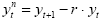
The superscript "n" indicates the values of the new, adjusted time course. The same calculation is also applied to each predictor time course resulting in an adjusted design matrix Xn. In the third step, the GLM is recomputed using the corrected voxel time course and corrected design matrix resulting finally in correct standard errors for beta estimates and to correct significance levels for contrasts. If autocorrelation is not sufficiently reduced in the new residuals, the procedure can be repeated.
While the AR(1) method for removal of serial correlations works well, it has been recently shown that a second-order, AR(2), model outperforms the AR(1) as well as other approaches currently used in fMRI data analysis. Since BrainVoyager QX 2.4, the AR(2) model is therefore used as the default approach to remove serial correlations from residual time courses in BrainVoyager QX; if desired, the simpler AR(1) model can still be specified. Note that the AR(2) model is turned on as default when calculating GLM analyses.
References
Draper and Smith (1998)
Kuttner, Neter... (2005)
Lenoski, B., Baxter, L. C., Karam, L. J., Maisog, J., and Debbins, J. (2008). On the performance of autocorrela- tion estimation algorithms for fMRI analysis. IEEE Journal of selected topics in signal processing, 2, 828–838.
Copyright © 2014 Rainer Goebel. All rights reserved.