BrainVoyager QX v2.8
EEG and MEG Forward Models
Introduction
Preparing a forward model represents the first step towards the reconstruction of the spatio-temporal activity of the neural sources of EEG or MEG data. This step involves computing the scalp potentials or the external magnetic fields at a finite set of electrode or sensor locations and orientations (called channel configuration) for a given predefined set of source positions and orientations (source space).
Assuming a channel configuration of M points and a source configuration of N points, in the most general case of a free orientation distributed source model, we have to fill out 3*N maps (one map per source location and source orientation in the 3D space) defined across the M channel sites. When, besides the location, the orientation of a source is also fixed (constrained orientation), we have N maps for N sources defined across M channel sites. These maps are called lead fields and by definition represent the field distribution across all M channels due to a unitary current dipole placed with a given position and orientation.
Background
Following Mosher et al. (1999), a convenient formulation of the EEG/MEG forward model entails with factorizing the electric field potential or the magnetic field observed at one extra-cranial point as the product of a "field kernel" and the dipole moment of the intra-cranial source (q). For (scalar) electrical potentials (v), the field kernel is a 3x1 vector (k); for (vectorial) magnetic fields (b), the field kernel is a 3x3 matrix (K):
In (1), r and rq represent respectively the positions of a channel site and of a source point. Thereby, computing a lead field for a given channel site and source position and orientation, entails with specifying q as a unit vector along the given orientation and replacing the coordinates of the channel and the source.
Spherical head model
A very common approximation in forward modeling consists in assuming the head is a set of nested concentric spheres, each corresponding to a layer. Typically, not more than four layers are assumed, corresponding (from the innermost to the outermost) to the brain, the CSF, the skull and the scalp. Assuming that each spherical layer has uniform and constant conductivity, rapidly computable analytic solutions exist for both EEG and MEG forward problem.
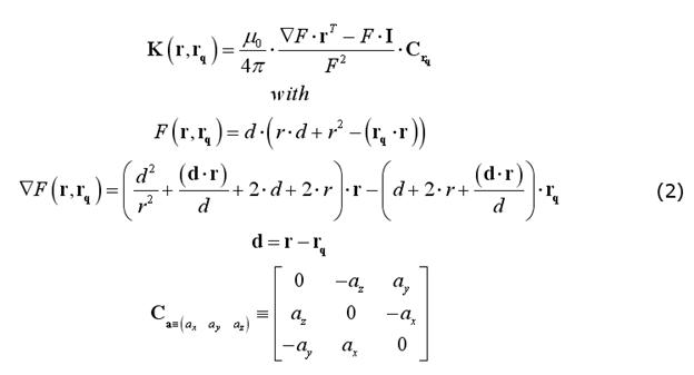
A very practical formulation of the EEG and MEG field kernels has been presented by Mosher et al. (1999), that only requires vectors expressed in their cartesian form. For MEG, since the magnetic permeability does not change across layers (and does not change much from the vacuum) and no currents exist outside the head (where the sensors are located), the full magnetic field outside a set of concentric spheres can be calculated without explicit consideration of the volume currents. Therefore, the MEG spherical model does not require specifying (or assuming) the number of and the radius ratios between the spherical layers and the field kernel can be computed as (Sarvas full MEG model):
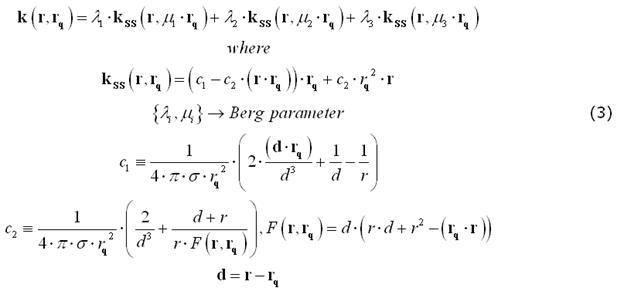
For EEG, the number and radii of the spherical layers are to be specified. Nonetheless, previous empirical work on closed-form approximations by Berg and Scherg (1994) and related theoretical studies by Zhang (1995) have gathered a valid and convenient method for approximating an EEG field kernel from a multi-layer spherical model as the weighted sum of three kernels from a single-layer spherical model applied to a modified source configurations. The optimal values of the "Berg parameters" (Eccentricity and Magnitude) in this approximation depend on the layer radii and conductivities:
Realistic head model
A more realistic head model requires that the real geometry and conductivity of the head layers be taken into account as much as possible. For real (non-spherical) geometry and conductivity fields, numerical solutions for the Maxwell equations are to be computed.
Assuming a piecewise constant distribution of the conductivity field, approximate, yet efficient and accurate, numeric solutions can be obtained for a realistically shaped head model using the so called Boundary Element Method (BEM). For BEM solutions, an MRI-based simplified description of the geometry is needed for computing the lead fields, and this can be provided in terms of (strictly) nested and closed surfaces corresponding to the boundaries separating the main tissue compartments (also called layers).
In practice (see application below), BEM solutions will only require to set a few conductivity parameters (one per tissue), and to specify a few triangular meshes, as can be obtained, e. g., with 3D volume segmentation tools from anatomical MRI data (VMR), each representing a separate interface between layers.
Application
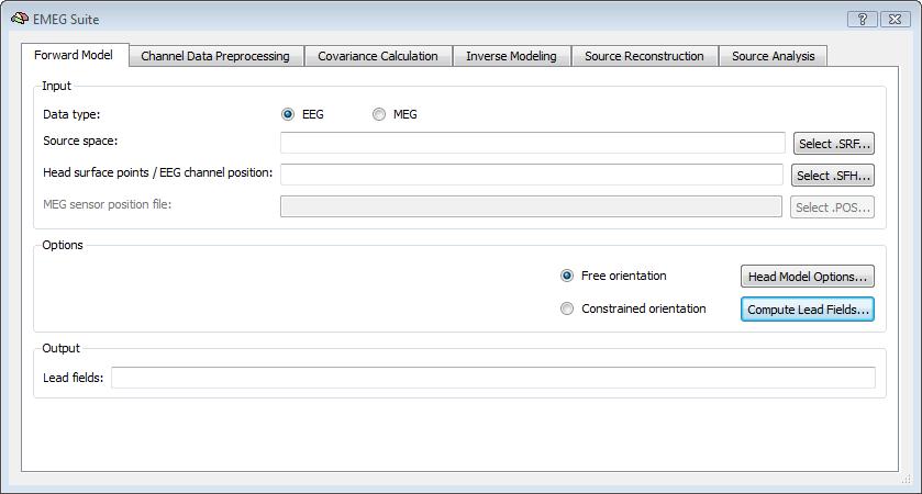
In BrainVoyager QX, it is possible to compute the EEG/MEG lead fields for a given configuration of the channel/sensor and source spaces, starting from either analytical solutions (using a spherical head model and the formulations (1) and (2) above) or numeric solutions (using the BEM solution). Besides the data type (EEG or MEG), the source space needs to be preloaded and selected as the default (current) cortical surface mesh. Moreover, the channel configuration needs to be specified via the list of (registered) head and surface points (SFH) and, for MEG only, the list of sensor positions and orientations (POS).
Please note: For EEG configurations, all head surface points (with the exclusion of the first three points, considered as fiducial points) are used for both head-surface registration and definition of the channel space (i. e. all surface points from 4 to N are interpreted as scalp electrodes). With this input, BrainVoyager QX can estimate either a free or constrained orientation forward model by computing the set of lead fields as SMP maps in the first tab of the EMEG Suite dialog:
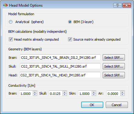
Even if the default head model is set to spherical, a 3-layer BEM solution can be computed (and the corresponding lead fields for a given configuration determined) by preparing three layer meshes for the standard compartments (brain, skull and head), and selecting the corresponding SRF files in the head model options of the EMEG suite (push button: Head Model Options...). When the BEM option is selected, the conductivity values for all compartments (brain, skull, skin and air) can be freely adjusted. However, apart from rare exceptions and special situations, it is always adviced not to change these values from their default settings, and in all cases, the changed values will only affect BEM solutions and not analytical solutions.
Important note: When selecting the BEM option and launching the lead field computations, the EMEG suite does not use only internal routines but produces a series of system calls to an external package called OpenMEEG. The OpenMEEG processor (copyright: INRIA, ENPC) is a powerful and accurate forward problem solver contributed by G. ADDE, M. CLERC, A. GRAMFORT, R. KERIVEN, J. KYBIC, P. LANDREAU, E. OLIVI and T. PAPADOPOULO, which has been made freely available as precompiled multi-platform binary packages on the web http://openmeeg.gforge.inria.fr. For contact and support about OpenMEEG, please send an email to: openmeeg-info@lists.gforge.inria.fr. NOTE: To make sure OpenMEEG is available on your system prior to running the calculations, please follow the following three steps: (1) go to the OpenMEEG website and download the OpenMEEG package setup (version 2.1, 32-bit is recommended for all platforms and both BV 32-bit and 64-bit versions), (2) run the set up wizard and read the licence information and (3), when prompted, do not forget to add OpenMEEG to your system path to make sure that all future BV calls will actually find the program regardless of where you copy the files.
The OpenMEEG approach is based on an extended version of the Green representation theorem, allowing for a special BEM formulation of the forward problem called the Symmetric Boundary Element Method. For all theoretical and implementation details, please read (and refer to) the following two publications: (1) Kybic et al. IEEE Transactions on Medical Imaging, 24:12-28, 2005 and (2) Gramfort, et al. BioMedical Engineering OnLine 45:9, 2010.
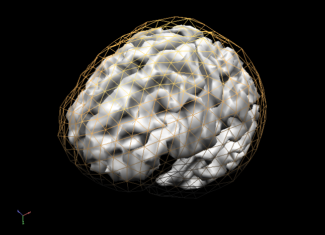
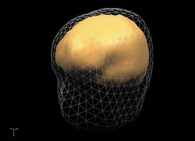
In order to succesfully compute EEG or MEG leadfields, four strictly nested and closed meshes should be made available in the current primary folder prior to running the calculations: (1) the source space mesh, (2) the brain layer mesh, (3) the skull layer mesh and (4) the head layer mesh. It is crucially important that all these meshes are perfectly nested with respect to each other, i. e.: all source space vertices (representing the source positions) are to be located inside the brain layer mesh, all brain mesh vertices are to be located inside the skull layer mesh and all skull layer mesh vertices are to be located inside the head mesh. When displaying these meshes as multiple scenes in the surface module you can toggle the filled vs wired display mode to see if this is the case.
Note: OpenMEEG functions always perform a detailed check of all meshes and will not produce any results in case the meshes are too irregular and do not strictly respect the above rules. To avoid extensive computations and to more easily produce regular nested meshes it is strongly advised to use very low resolution source (see also practical tips below) as in the examples below showing a correct brain mesh and a correct skull mesh.
The BEM forward model calculations are performed in three separate steps: (1) head matrix calculation, (2) source matrix calculation and (3) lead field calculation.
Step (1) (head matrix calculation) is only based on the head geometry model and therefore the results will be only dependend on the three layer meshes and the chosen modality (EEG or MEG), but will be the same regardless of the position of the sources and the channels. As a consequence, the same head matrix can be re-used if the same layer meshes are specified, when recomputing the lead fields for a different source space and/or for a different channel configuration. When the head matrix is computed once for a given set of layer meshes, two files are written to disk called "tmp.hm" and "tmp.hm_inv" containing the head matrix and its inverse which can be possibly re-used for a new BEM calculation that skips this step. When the head matrix has been already computed, and the user expressely requires these calculations not to be repeated by checking the option "Head matrix already computed" in the dialog, the program assumes that the "tmp.hm" and "tmp.hminv" files are present in the current folder and compatible with the layer meshes (that need to be specified anyway). If this is not the case, an error will occur and no lead fields will be computed and returned.
Step (2) (source matrix calculation) is only based on the head geometry and the position of the sources, and therefore the results will be only dependent on the three layer meshes, the source space mesh and the chosen modality, but will be the same regardless of the position of the channels. As a consequence, the same source matrix can be re-used if the same head matrix, and the same layer and source meshes are specified and selected, when recomputing the lead fields for a different channel configuration. When the source matrix is computed once for a given set of layer meshes and a for a given source space mesh, either three files ("Xtmp.dsm", "Ytmp.dsm", "Ztmp.dsm") or just one file ("Ntmp.dsm"), are written to disk in the current folder, depending on whether a free (default) or a normally constrained orientation model is selected for the sources. When the source matrix has been already computed, and the user expressely requires these calculations not to be repeated by checking the option "Source matrix already computed" in the head model options dialog, the program assumes that the "X/Y/Z/Ntmp.dsm" are present in the current folder and compatible with the layer and source meshes (but the layer meshes need to be specified anyway). If this is not the case, an error will occur and no lead fields will be returned.
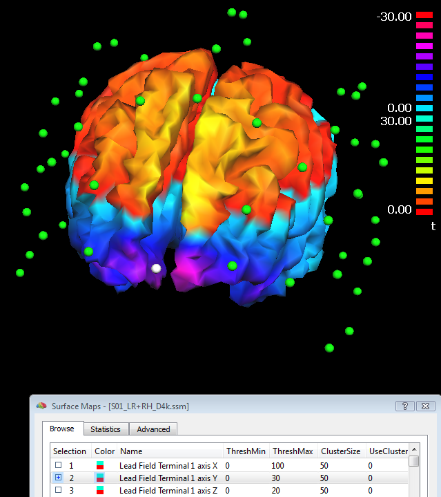
Step (3) (lead field calculation) is repeated every time the button "Compute lead fields..." is pressed in the Forward tab of the EMEG suite and, if no errors occur because the geometries are correct or compatible with each other, the lead fields are returned in the resulting surface map (SMP) file. In addition to the SMP file, a dipole (DPL) file called "Terminals.dpl" is also written to disk, allowing a display of the last channel configuration used in the last lead field calculations. This DPL file can be edited and loaded from the EEG-MEG menu where it can be used to display the channels and sensons together with the lead field maps, as illustrated in the figure below (where channel 1 is colored in white). For practical reasons, BrainVoyager QX represents the set of lead fields in a "reciprocal" fashion, i.e. as 3*M (for free orientation models) or M (for constrained orientation models) surface maps defined across all source points (vertices), M being the number of channels. It is always possible to rank-reduce the lead fields from 3 to 2 dimensions spanned, but (for compatibility issues) the three cartesian dimensions are written with all 3 coordinates of the internal coordinate system.
Practical tips for individual head model preparation
In order to prepare individual head BEM models from MRI images, a number of segmentation tools can be used and some morphological operations can be performed in the volume (base) module of BrainVoyager QX.
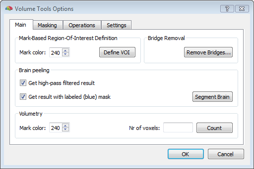
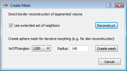
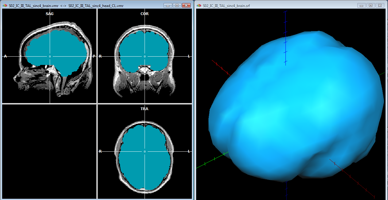
To start, a good quality, inhomogeneity corrected and background cleaned VMR should be created (and preprocessed) from 3D T1-weighted MRI images covering the entire head. With these prerequesites, the options of the 3D segmentation tools (Segmentation tab-> options) can be invoked to perform standard brain peeling and getting the result as a blue-labeled volume mask. To get the brain volume labeled, this option should be expressely set (see figure below). Then, after setting to zero all non-marked voxels, from the meshes menu, a simple low-resolution (e. g. with 1280 triangles) sphere mesh can be created and iteratively morphed until fitting the boundary of the brain compartment, as illustrated in the example below.
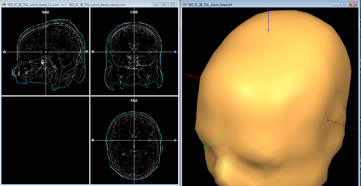
In order to reasonably approximate the head and skull layers, it may be convenient to apply a canny edge detection filter to the original (clean) whole-head VMR, and saving the result to another VMR. This additional VMR may help to best identify the boundary of the scalp (which can be used to guide the head layer definition) and the boundary of the dura matter (which can be used to guide the skull layer definition) as illustrated below. Unfortunately, standard 3D T1 MRI images do not allow to easiy segment the skull bone directly, and therefore, unless a 3D CT scan is available for the same subject, an indirect approach is to be used.
For the head layer, starting from the whole-head (cleaned) VMR, and growing a region covering the entire head, a good approximation of the head layer can be easily obtained by creating a low resoluton sphere mesh and morphing this until fitting the boundary of the segmented head. Loading the edge-filtered VMR as secondary VMR, and toggling the double VMR view with F8/F9 keys, allows to compare the boundary of the segmented volume with the detected edges on the original VMR.
Important note: while using a low resolution mesh is adviced for the BEM head layer mesh creation and morphing, this is not the case for channel and surface point head (SFH) registration. For registration, it is much better to use to high resolution head mesh as this meshes will gather a better fitting of the electrode and surface points. On the other hand, using high resolution head meshes are BEM layer meshes may lead to prohibitevely extensive calculations and errors.
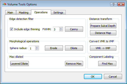
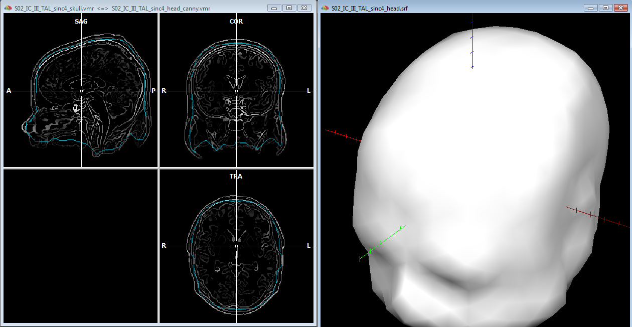
After saving the head mesh to disk, one can continue with the same segmentated volume (and the same reconstructed mesh) to approximate the skull layer with another mesh. In the volume space, while keeping an eye on the correspondence between the volume boundary and tissue edges, one can apply a few "erode" steps to the current segmented volume and a few morphing iterations to the current mesh, until a reasonable approximation of the skull layer is achieved (see example below). Of course, as anticipated, this MRI-based only approximation can be rather crude, however, the solution is often acceptable as the shape of the skull follows that of the skin much more than that of the brain, thereby the erode-based approach applied to the head layer should be slightly preferred to a dilation-based approach applied to the brain layer. Moreover, the suggested approach allows to quickly obtain a set of individually shaped and strictly nested BEM layer meshes, for their use in the forward modeling, and anyway it is possible to manually refine the segmented volume using all other 3D segmentation tools.

References
Berg, P., Scherg, M., 1994. A fast method for forward computation of multiple-shell spherical head models. Electroenceph. Clin. Neurophysiol., 90, 58-64.
Gramfort, et al. BioMedical Engineering OnLine 45:9, 2010.
Kybic et al. IEEE Transactions on Medical Imaging, 24:12-28, 2005.
Mosher, J. C., Leahy, R., Lewis, P., 1999. EEG and MEG: forward solutions for inverse methods. IEEE Trans Biomed. Eng. 46, 245-259.
Sarvas, J., 1987. Basic mathematical and electromagnetic concepts of the biomagnetic inverse problems. Phys. Med. Biol., 32, 11-22.
Zhang, Z., 1995. A fast method to compute surface potentials generated by dipoles within multilayer anisotropic spheres. Phys. Med. Biol., 40, 335-349.
Copyright © 2014 Fabrizio Esposito and Rainer Goebel. All rights reserved.