BrainVoyager QX v2.8
Regular 2D Grids At Different Cortical Depth Levels
While the described whole-mesh cortical depth sampling tool can be used to sample functional (and other) data from different cortical depth levels, the unregular spacing of the vertices of a standard reconstructed mesh will lead to suboptimal geometric sampling (for details see Issues of whole-mesh cortical depth sampling); In order to further improve cortical depth sampling, a second sampling approach is presented here that creates separate regular two-dimensional grids at any specified relative cortical depth level for geometrically accurate sampling of high-resolution (sub-millimeter) functional data. While this tool produces more precise sampling results than the whole-mesh sampling approach, it is only suited for small grey matter regions extending a few centimeter along the cortex.
Background
As the whole-mesh sampling tool, the regular grid cortical depth sampling approach is also built on information obtained from the cortical thickness measurement tool. The VMR data set used for these tools should be of high-quality (i.e. high grey/white matter contrast) and with sub-millimeter (measured or interpolated) resolution, preferentially at 0.5-0.8 mm. Using the cortical thickness mesurement maps as input, a gradient value pointing in the direction of cortical depth is extracted at each grey matter voxel. Integrating along these gradient values produces "field lines" or "streamlines" (Jones et al., 2000) as used in cortical thickness calculations to travel from the white / grey matter boundary to the pial surface (or vice versa). For constructing a grid at a fixed relative depth level ("equipotential surfaces", Jones et al., 2000), step sizes are performed orthogonal to the streamline gradient in two orthogonal directions resulting in regularly spaced grid sample points at a given relative depth value. If, for example, the initialized depth value is 0.5, one grid axis will be created along the first chosen direction (prime direction vector) that traces a (curved) line at a constant depth level through the middle of grey matter; at regular intervals along this first line, additional lines will be started in orthogonal direction (secondary direction vector) providing regularly spaced grid points along the second axis at the same relative depth level. Note that the traversal through grey matter requires information of the cortical thickness maps (thickness values and x/y/z gradient values) at arbitrary 3D coordinates, which is obtained by trilinear interpolation from neighboring voxel values. The emerging grid is constantly fine-tuned to assure that horizontal and vertical distances are kept constant forming extended regular grids that can be subsequently used to topographically sample aligned functional and other data sets.
Creation of Grids - Two Approaches
In the equal local distance version, the described procedure is performed for each desired relative depth level resulting in grids with precise geometrical information about distances and surface area along folded cortex patches at different relative depth levels. Since spacing between grid points is identical in different grids, the extent of covered cortex may be different, however, since it depends on local curvature. The equal cortex coverage version (default) uses calculated streamlines that precisely relate corresponding grid points across multiple cortex depth levels. In this approach, the grid sampling tool creates first a regular spaced grid at the middle layer of the cortex and then creates subsequent grids by moving up or down grid points along streamlines to get corresponding grid points for other relative depth levels. Note that in this approach distances between points in grids at depth levels unequal to 0.5 will not be exactly identical but will be squeezed or expanded a bit with respect to local curvature.
Mapping Functional Data on Sampled Grids
The coordinates of the grid points of a created regular grid are then used to sample functional data from attached high-resolution volume maps. The sampled values are shown in 2D plots as well as directly at corresponding 3D points in the surface view. The latter possibility allows to inspect how the mapped functional data extents along curved cortex at different depth levels.
While the result of cortical depth sampling roughly corresponds to sampling different cortical laminae, it is important to note that the relative position of laminae within the cortex depends to some extend on the curvature of the cortex, i.e. the relative position of a cortical layer is different at the fundus of a sulcus as compared to the crown of a gyrus. An optional (approximate) correction for this curvature-based lamina depth dependence is planned for a future release.
Application
After loading a high-resolution (preferentially 0.5 - 0.8 mm) VMR data set, the High-Resolution Cortex Grid Sampling dialog (see snapshot below) can be launched by clicking the High-Resolution Cortex Grid Sampling item in the Volumes menu. There are two possibilities to specify the region where grids should be calculated in the brain. The easiest posssibility (available since BrainVoyager QX 2.8.2) is to provide a volume-of-interest (VOI) from which the program derives all necessary information automatically to start the grid construction process. The second possibility is to provide a 3D reference point around which the grids should be sampled; in the latter approach one must also explicitly specify the size of the grids and a direction vector telling the program in which direction to sample from the reference point. Since the coordinates of the 3D point are determined from the current position of the 3D cross within a VMR data set, it is important to set the cross position prior to entering the High-Resolution Cortex Grid Sampling dialog since the cross position can not be changed as long as the dialog is open. Furthermore, the cross needs to be positioned in grey matter, otherwise grid sampling will not work. Note that the resulting grids will be roughly centered around the chosen reference point in the VMR data, i.e. the cross position is interpreted not as a grid corner point but as the center of the grids.
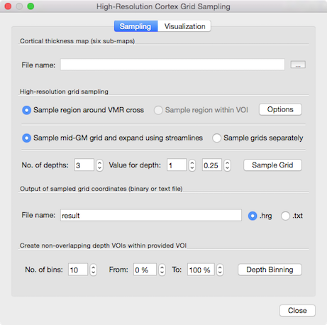
The snapshot above shows the High-Resolution Cortex Grid Sampling dialog. The invoked dialog contains two tab pages, Sampling and Visualization. The Sampling tab (shown above) is used to specify the parameters for the grid creation procedure while the Visualization tab is used to visualize the obtained grids optionally with mapped functional data from a specified high-resolution volume map. To enable grid sampling, a cortical thickness map for the current VMR data set has to be loaded using the Browse ("...") button on the right side of the File name text box in th Cortical thickness map (six sub-maps) field. As described above, grids can be created for a specified VOI or around a provided 3D reference point.
Grid Sampling In Specified VOI
The easiest way to sepcify what region should be used for the creation of regular grids is to provide a volume-of-interest (VOI). In case a VOI file has been loaded prior to entering the High-Resolution Cortex Grid Sampling dialog, the Sample region within VOI option will be enabled and can be selected. If a VOI file has not been loaded, the option is not availalbe (greyed out) and one needs to click the Options button on the right side to specify a VOI file in the Grid Sampling Region dialog.
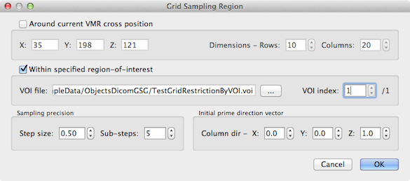
When the dialog appears and no VOI file has been specified earlier, the Around current VMR cross position option is selected as default (see below for a description of this approach). To specify a VOI file, the Within specified region-of-interest option needs to be enabled (checked). In the example snapshot above, the "TestGridRestrictionByVOI.voi" file has been selected in the appearing File Open dialog. In case that the VOI file defines coordinates for more than one VOI, you can select the desired one using the VOI index spin box (the first VOI is always selected as default). No further setting is required for this approach to specify the region for grid construction. You may, however, adjust the values in the Sampling precision field if desired. The Step size spin box sets the distance between neighboring horizontal and vertical grid points. The default value of 0.5 specifies that the grid will be constructed with a spatial sampling resolution of 0.5 voxels. During the grid creation process, even smaller steps are made to follow equipotential lines and streamlines with high precision. This sub-sampling precision can be influenced by changing the value in the Sub-steps spin box; the given value specifies how many sub-sampling steps will be performed until a point of the constructed grid is reached. With the default settings of 5 sub-steps (recommended) and a desired grid spacing of 0.5 voxels, the actually executed sampling step size is 0.5 / 5 = 0.1. After pressing the OK button, the grid sampling process can be started by clicking the Sample Grid button in the High-Resolution Cortex Grid Sampling dialog.
The program will use the voxel coordinates of the specified VOI and attempts to create grids at specified depth levels that optimally cover the defined region. Since the resulting grids are always two-dimensional, the covered region will usually not precisely cover the given VOI. In order to determine the most optimal directions for the two dimensions of the grids, the program uses the following approach. First, the border voxels of the specified VOI are determined and border voxels outside grey matter are ignored, i.e. VOIs need not to be perfectly defined within grey matter since white-matter/CSF voxels are removed automatically. From each grey matter voxel at the border of the VOI a direction vector is determined that points inside the VOI. Using this direction vector, a path is traversed through grey matter until a voxel outside the VOI is reached. The program selects the voxel that led to the longest path as a reference point for subsequent grid creation with the direction through the VOI as the first axis of the resulting grids. While the voxel with the associated longest path through the VOI determines one dimension of the grids, it does not provide information about the width of the grids. In order to get a useful width value, the program moves to the center point of the determined longest path. Since this point should be roughly located in the middle oft the VOI, the program now moves orthogonally (to the "left" and "right") to find the width of the second grid dimension. This procedure is a heuristic that works well if the VOI shape has two rather constant dimensions ("width" and "height"). If the VOI has a wider extension in the middle than at the borders, the resulting grids will extent beyond the VOI at the borders but will still cover the VOI completely. If the VOI is taller in the middle than at the borders, the grids might not cover the extent of the VOI along the cortex completely.
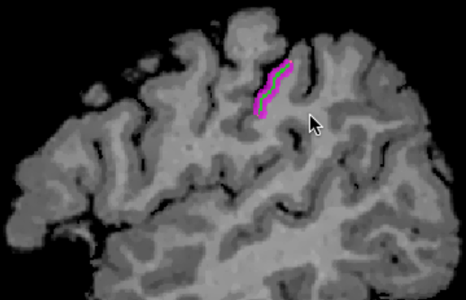
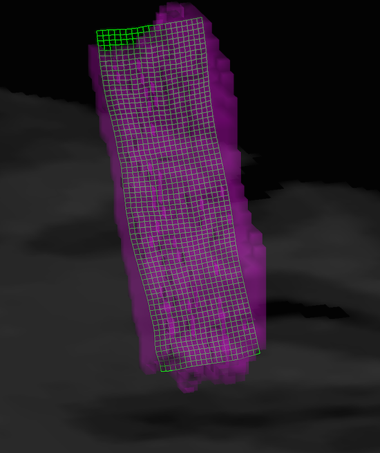
The example snapshot avove shows a sagittal slice through a defined VOI (magenta colors) that extends mainly in the superior-inferior direction while the extension in the left-right dimension is much smaller (not visible on sagittal slice). The green line indicates one of the reconstructed grids that runs through the middle of grey matter (depth level 0.5). As can be seen, the long dimension of the grids covers the VOI well. The sanpshot below shows the VOI as a transparent mesh (magenta color) in the surface window together with the same mid-level grid (green color). The 3D view is in the anterior-posterior direction revealing that also the "width" of the VOI is covered well by the grid creation strategy.
Details about visualization options of reconstructed regular grids are provided below in the section "Grid Visualization".
Grid Sampling Around 3D Point
The Rows and Columns spin boxes in the High-resolution grid sampling field control the resulting dimensions and resolution of one or more grids created at specified relative depth levels. The distance between neighboring horizontal and vertical grid points is specified in the Step size spin box. The default value of 0.5 specifies that the grid will be constructed with a spatial sampling resolution of 0.5 voxels. During the grid creation process, even smaller steps are made to follow equipotential lines and streamlines with high precision. This sub-sampling precision can be influenced by changing the value in the Sub-steps spin box; the given value specifies how many sub-sampling steps will be performed until a point of the constructed grid is reached. With the default settings of 5 sub-steps (recommended) and a desired grid spacing of 0.5 voxels, the actually executed sampling step size is 0.5 / 5 = 0.1. Note, however, that this step size calculation is only strictly valid for the equal cortex coverage version (see above). This version can be chosen by checking the Sample grids separately option. When using this version, the created grids at different depth levels will have the same absolute extent in the two grid dimensions. Because of local curvature, grids at inner or outer depth levels may be, however, substantially shorter or longer than grids at middle depth levels. While this may be desirable for some applications, it is often more important that successive grid points at different depth levels correspond to each other along streamlines across depth levels. This implies that the distance between grid points will be smaller in lower depth levels than in higher depth levels in regions with convex curvature (e.g. gyri) and vice versa in regions with concave curvature (e.g. sulci). This equal cortex coverage approach is used in case that the Sample mid-GM grid and expand using streamlines option is turned on (default). This depth sampling version is particularly useful if one wants to evaluate activity at different depth levels for corresponding positions, e.g. in the context of columnar-level imaging (Zimmermann et al., 2011). With this option, the x, y coordinates of a position in all resulting depth-level grids corresponds to the same tangential cortex positon (as defined by streamlines).
The number of desired grids (default: 3) is specified in the No. of depths spin box. For each desired depth level a relative depth value can be provided in the right spin box of the Value for depth pair of spin boxes. Use the left spin box to select one of the relative depth grids and enter a relative depth value in the right spin box. As default three grids are specified with relative depth values of 0.25, 0.5 and 0.75. While the start position of grid sampling is determined by the location of the cross in the VMR view, the direction used for grid sampling is specified using the X, Y and Z spin boxes at the right side of the Initial prime direction vector (column dir) label; the three spin boxes determine the components of the vector with respect to system coordinates, i.e. the x coordinate moves from left to right in the coronal/axial planes (which is from right-to-left positions in the brain for the default radiological convention), the y coordinate moves from front to back (anterior to posterior) and the z coordinate moves from top to bottom (superior to inferior). For the default prime direction vector 0.0, 0.0, 1.0, for example, grid sampling would move in the superior to inferior direction; the specified direction describes the desired direction of the columns of the grid. Note, however, that the provided prime direction vector is considered only as a hint for the determination of the actually used direction since the used direction vector is always forced to be orthogonal with respect to the gradient direction (streamline) at a visited location. Note also that dependent on the curvature of the sampled region, the prime (column) direction vector as well as the internally calculated secondary (row) direction vector will be updated at each sampled location in such a way that they both are always orthogonal to each other as well as orthogonal to the current streamline gradient direction pointing from the white / grey matter to the grey matter / CSF boundary. In addition to these constraints, a visited location is forced to be at a grid's relative depth level within grey matter.
Output: Coordinates of Sampled Grid Points
To start the grid construction process, click the Sample Grid button; the coordinates of the sampled grid points will be stored for each depth grid in working memory and also saved in a file for later use in BrainVoyager and for custom processing (e.g. in Matlab); the grids can be saved as a binary file (default) by turning on the hrg (high-resolution grid) option or as a text file by checking the txt option in the Output of sampled coordinates field. The format of the text file is as follows:
FileVersion:  f [file version, only version 1 supported at present]
NrOfGrids:    D [No. of grids]
DimY:         Y [No. of grid rows]
DimX:         X [No. of grid columns]

AcrossPathStepSize: ys [step size in y direction]
WithinPathStepSize: xs [step size in x direction]

[Loop d: No. of grids]
    [Loop y: No. of grid rows]
        [Loop x: No. of grid columns]
            x-coordinate of grid-point x, y, d
            y-coordinate of grid-point x, y, d
            z-coordinate of grid-point x, y, d
        [Loop x end]
    [Loop y end]
[Loop d end]

[Loop d: No. of grids]
    NameOfGrid-d: [Name of grid in parantheses]
[Loop d end]
The binary (.hrg) file follows the same structure but does not save any explanatory string, i.e. the values of the variables are stored in consecutive order (little endian byte order); the value of the file version is a 2-byte integer, while the values of the number of grids, grid rows and grid columns are 4-byte integer values. The across path step size and within path step size values as well as the x, y, z, coordinate values of each grid point are 4-byte float values. The names of the grids are stored as 0-terminated C strings at the end of the file.
Binning Voxels in Separate Depth VOIs
While 2D grids are useful to sample topographic functional information along the cortex, the grids in different depth levels will use the same voxels to some extent when sampling the data. For some applications, for example to detect layer-specific attentional effects, the exact topography might not be critical but it might be important to completely segregate the voxels assigned to different depth levels. This latter application can be achieved by using the Depth Binning button in the Create non-overlapping depth VOIs within provided VOI field. This function (introduced in version 2.8.4) will assign each included grey matter voxel in a provided VOI (see above) to a different depth bin as specified by the No. of bins spin box and the overall depth interval as specified with the From and To spin boxes. If, for example, the whole grey matter should be included, the interval should be specified (default) from value 0% (white matter - grey matter boundary) in the From spin box to value 100% (grey matter - CSF boundary) in the To spin box. It might be, however, better to use a safety margin and change these values, e.g. from 10% to 90% relative depth. The specified depth range is partitioned in as many bins as specified in the No. of bins spin box, i.e. the size of each bin will be: (to - from)/n_bins. If, for example, 10 bins are used to segregate the voxels within a depth range from 0% to 100%, the bin size will be 10%; or if, for example, 3 bins for a depth range from 10% - 90% is used, the bin size will be 26.7% and the first bin would start at 10% depth.
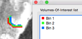
After clicking the Depth Binning button, the program will use the provided cortical thickness maps to extract the relative depth value of each voxel in the provided VOI. Each voxel within the specified depth range will then be assigned to the respective depth bin. This procedure ensures that the created sub-VOIs contain non-overlapping depth bins. The figure above shows the separation of a provided hMT VOI into 3 sub-VOIs (Bin 1, Bin 2 and Bin 3) in the 0% -100% range, visualized on a coregistered functional scan. All standard VOI tools can now be used to extract (statistical) map data or time course data from the non-overlapping bins. This can be, for example, useful to study layer-specific connectivity, layer-specific classification and layer-specific attentional effects. Additional information about the bin size and the number of voxels in each bin is printed into the Log pane; for the example shown above, the following output is generated:
Depth binning: bin size = 0.333333
Histogram - number of voxels per depth bin:
bin 1: 365
bin 2: 299
bin 3: 222
References
Jones, S.E., Buchbinder, B.R., Aharon, I. (2000). Three-Dimensional Mapping of Cortical Thickness Using Laplace's Equation. Human Brain Mapping, 11, 12-32.
Copyright © 2014 Rainer Goebel. All rights reserved.