BrainVoyager QX v2.8
pRF Estimation in Cortical Surface Space
The Fit pRFs tab of the Population Receptive Field dialg is used to find the population receptive field model that best explains the measured fMRI time courses of provided input data. If the dialog is called from a mesh document (surface) window, the Fit pRFs tab adjusts some of its fields to handle SRF-MTC projects.
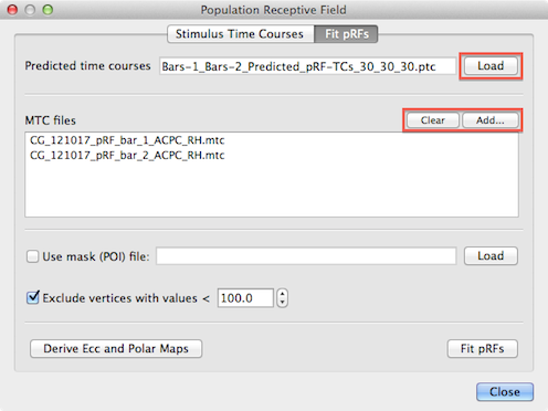
To run the pRF fitting procedure, the program needs as one input source the model time course created earlier with the Stimulus Time Courses tab. The Load button on the right side of the Predicted time courses text field (see snapshot above) can be used to load a desired .ptc file; note that this field might be already filled in case one moves straight to the Fit pRFs tab after having generated time courses in the Stimulus Time Courses tab.
Furthermore, the program needs to know the MTC files that contain the measured fMRI time course data. One or more MTC files can be added to the MTC files list using the Add button (see snapshot above). Note that in case that multiple runs are analyzed, the order in which the MTC files are added here needs to match the order in which the stimuli have been added in the Stimulus Time Courses tab to generate the .stm file. For the used example, two MTC files have been added containing the measured fMRI data of the two experimental runs where bar stimuli had been presented.
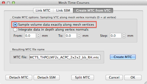
In order to obtain cortex mesh time course (MTC) files, standard cortex segmentation routines should have been applied to obtain cortex meshes followed by the standard VTC-to-MTC conversion routine available in the Create MTC from VTC tab of the Meshes Time Courses dialog; in order to optimally separate activity at two opposing banks within sulci in the occipital lobe, it is recommended to use the Sample volume data exactly along mesh vertices option (see snapshot above) and to use the (linked) "_RECO" or "_RECOSM" version when creating the MTC file.
Since all (e.g. 27,000) model time courses are fitted in separate GLM's to each voxel of the SRF-MTC project, it is recommended to limit the number of considered mesh vertices to those in a mask containing the cortex of the occipital lobe. A subset of vertices can be specified for analysis by providing a patch-of-interest (POI). The Load button on the right side of the Use mask (POI) file text field (see snapshot below) can be used to load a previously prepared .poi file. A POI containing the occipital lobe can be easily specified on an inflated version of a cortex mesh using standard mesh drawing and filling tools. Another possibility to get a useful mask is to run a standard GLM contrasting stimulation periods to baseline (fixation) periods. This requires creation of a corresponding protocol (.prt) file; the resulting statistical map can be converted into one or more POIs by using the Convert button in the Create POIs from map clusters tab of the Surface Maps dialog. Note that it is recommended to have only one POI defined in the .poi file - if more than one POI is defined, the first one will be used. In the snapshot below, the prepared .poi file "Occ_RH.poi" has been loaded for analysis of the right cortex hemisphere; a similar file has been prepared also for the left hemisphere. While not demonstrated here, it is also possible to merge the left and right hemisphere cortex meshes and to create (or merge) a single MTC file (per run) for the whole cortex. The example analysis described uses the more common case in which each hemisphere is analyzed separately.
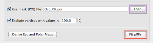
Besides spatial masking, vertices can also be excluded if they contain time course data with low intensity values likely corresponding to non-brain background voxels. This exclusion criteria is enabled by checking the Exclude vertices with values < option (turned on as default) and the threshold intensity value can be specified in the Intensity threshold spin box (value 100.0 is used as a reaonable default setting). While this option (see snapshot above) is not relevant when using a cortex mask, it may help to reduce the number of analyzed vertices when no POI mask is provided.
If the pRF model time course data, the MTC file(s) and optionally a spatial mask file have been provided as input, the population receptive field estimation can be started by clicking the Fit pRFs button (see snapshot above). For each vertex included in the analysis, a separate GLM is executed for each pRF model with the model's time course as the main predictor (predictor of interest) of the GLM design matrix X. For each run included in the analysis, a separate constant predictor is added to the design matrix (as in a multi-run GLM) allowing to fit a different beta weight for the baseline level. The time course data of a vertex is transformed into percent signal change values separately for each run and then concatenated providing the observed (to-be-explained) data y of the GLM. The GLM for each pRF model is calculated and the amount of explained variance R2 is recorded - the model that results in a GLM with the highest explained variance value is assigned as the pRF model for the considered vertex. This procedure is repeated for each vertex included in the analysis. The parameters of the best fitting model are stored in a surface map providing the final output of the fitting procedure, i.e. for each analyzed vertex, the pRF model's position in the visual field (x, y values) and the model's receptive field size are recorded in different sub-maps (see snapshots below) of the surface map data. The surface map is saved to disk automatically using an appropriate name containing the name of the mask file (if used) and number and range of pRF models used (i.e. the name will be similar as the one created for the .ptrc file).
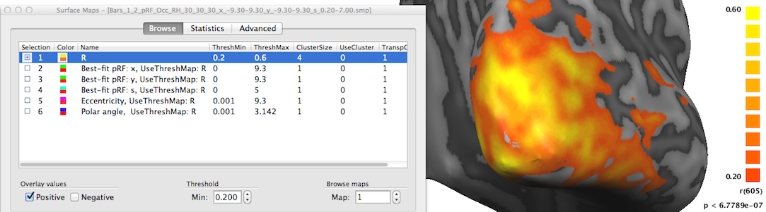
In order to inspect the estimated pRF data, open the Surface Maps dialog (see snapshot above). The dialog will contain six sub-maps. The first sub-map is a multiple correlation map named "R" (see snapshot above) containing the square root of the explained variance of the best fitting pRF model per vertex. This statistical map is instructive in itself but it is also used to theshold other maps that contain non-statistical values such as the location of the vertice's pRF in the visual field. Note that all other sub-maps contain the sub-string "UseThreshMap: R" in the map name. The "UseThreshMap" instruction string has been originally introduced in the context of "winner maps" to allow sub-maps containing qualitative (non-ordered categorical) values to use another map for thresholding. This mechanism has been extended to support that any kind of map can refer to any other map using it for thresholding. This provides the possibility for pRF model parameter maps as well as derived eccentricity and polar angle maps (see below) to show the full range of their values while still being able to remove noisy vertices by using the "R" map for thresholding. If the threshold (set to 0.2 as default) of the "R" map is changed, the effect will be visible when selecting one of the other sub-maps.
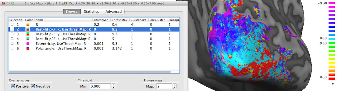
The second map "Best-fit pRF: x" contains the x location of the pRF model assigned to a vertex. As one would expect, mainly negative x values (representing pRF model locations in the left visual field) are visible on the shown right cortical hemisphere (see snapshot above); positive x values (right visual field) will be visible mainly on the left cortical hemisphere (not shown).
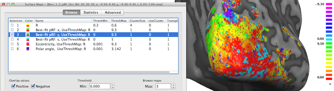
The third map "Best-fit pRF: y" contains the y location of the pRF model assigned to a vertex. In the snapshot above mainly positive values (red-yellow-green colors) are visible since the selected posterior view contains mainly visual cortex for lower visual field locations.
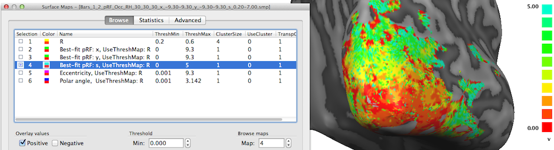
The fourth map "Best-fit pRF: s" contains the receptive field size of the pRF model assigned to a vertex. The red/orange colors around the occipital pole shown in the snapshot above indicate that receptive field sizes are small in these regions while in the more upper and lateral regions of the visible cortex contain larger receptive field sizes as indicated by the yellow/green colors. Note that it may be instructive to change the upper (display) threshold to a lower value than the default value (10.0) in order to better see small gradients of receptive field size changes, e.g. within areas V1/V2; in the snapshot above, the value has been set to 5.0 degrees.
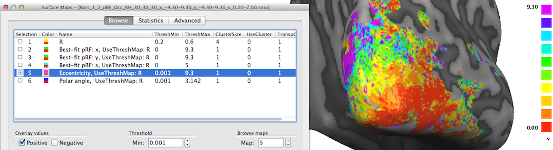
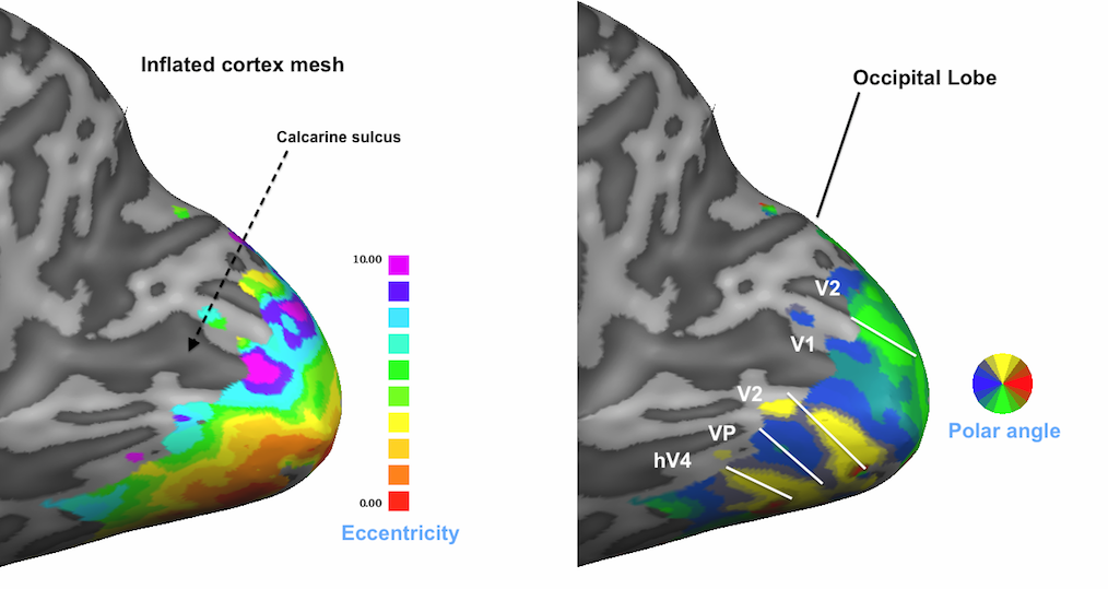
The maps described so far are direct representations of the population receptive field models fitted to the data. Sub-maps 5 and 6 contain eccentricity and polar angle values that are simply derived from the x and y pRF model parameter maps. These maps are added to provide visualizations of the obtained pRF results in the same way as in conventional phase-encoded retinotopic mapping experiments. The fifth map "Eccentricity" contains estimates of eccentricity values ecc that are simply obtained by applying the equation ecc = sqrt(x2 + y2) at each vertex. The snapshot above shows a clear eccentricity gradient as observed in conventional eccentricity mapping experiments.
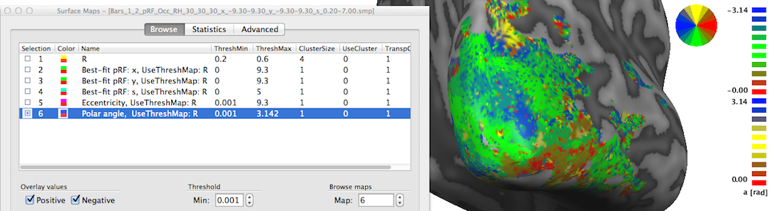
The sixth map "Polar angle" contains estimates of the location in polar coordinates; the calculated angle α is expressed relativ to the positive (right pointing) x axis and is simply obtained by applying the equation α = atan2(-y, x) at each vertex. Note that the sign of the value for the pRF y location is flipped (-y); this is done because the y axis in the implemented stimulus representation is defined from top (-) to bottom (+) while the coordinate system used in the unit circle of trigonometry runs from botton (-) to top (+). By flipping the y axis, the angles can be interpreted as in the unit circle, i.e. the angles are expressed with respect to the right half of the x axis (α = 0) and increase counter clockwise with α = 90 (π/2 radians) corresponding to the upper (-y) y axis, α = 180 (π radians) corresponding to the left half of the x axis and α = 270 (-π/2) is reached at the lower (+y) axis. In order to appropriately represent, process (e.g. spatially smoothing) and visualize angle maps, the map type "a" has been introduced in BrainVoyager where angles are expressed in radians with positive values for the upper half of the unit circle and negative values for the lower half of the unit circle. The snapshot above indicates below the color bar with the string "a [rad]" that the "Polar angle" map is represented as the new map type "angle". The positive and negative map maximum values "3.14" indicate (approximately) value π; furthermore, the color bar is also shown in a filled circle (disk) that facilitates relating colors in the map to angles, which is especially helpful when using polar angle maps to separate early visual areas from each other (see right side in snapshot below).
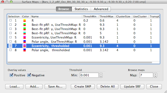
For the snapshot above, the eccentricity and polar angle maps have been spatially smoothed. In order to limit smoothing to the regions surpassing the threshold of the referenced threshold map "R", a version of the pRF and eccentricity/polar angle maps can be obtained where the values below the current threshold in the linked "R" map are set to 0.0. This linked mesh filtering function can be performed by clicking the Filter UseThreshMaps button in the Combine SMPs dialog after selecting one or maps with the "UseThreshMap" string. In the snapshot below, the resulting eccentricity and polar angle maps can be identified by the string "thresholded" that is automatically replacing the "UseThreshMap" substring when applying the filtering/masking.
The selected thresholded eccentricity map is shown below unsmoothed as well as after increasing amounts of smoothing by applying the Smooth SMP button in the Advanced tab of the Surface Maps dialog. The Restrict to vertices with value unequal 0.0 option (on as default) will exclude vertices that have a value of exactly 0.0 (that is usually interpreted in BrainVoyager as a "missing value" entry). This has the desired effect to limit smoothing to the relevant regions. Futhermore the Restrict to neighbors with value unequal 0.0 option ensures that a smoothed vertex will not include the values of those neighboring vertices into account that have exactly the value 0.0. This is an important option avoiding that vertices at the "fringe" of the active regions are not artifically biased towards low values which would happen when one would include neighbors with 0.0 values.
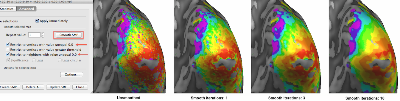
This option is also important when one deliberately wants to expand the map to vertices with 0.0 values, e.g. when one aims to close "holes" in the map since than vertices with 0.0 values will only include the values of neighbors with non-zero values. This can be achieved by turning off the Restrict to vertices with value unequal 0.0 option but not the Restrict to neighbors with value unequal 0.0 option.
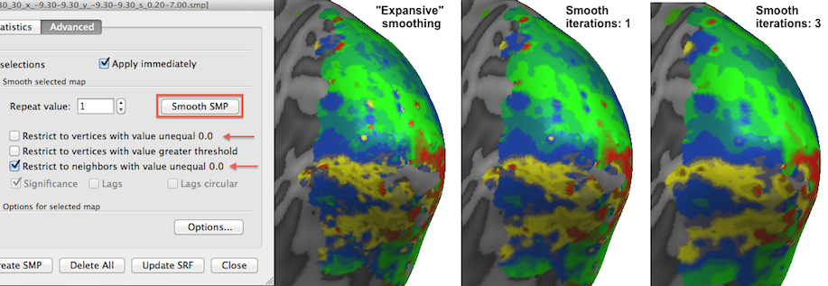
The snapshot above shows the result of this "expansive" smoothing; the right version of the map (3 iterations of expansive smoothing) clearly has invaded somewhat into regions that had 0.0 map values in the version of the map shown on the left side. It is usually not recommended to use expanding smoothing since it pretends that vertices have values which actually did not show values under a given threshold, but for visualization purposes one (or a few) expanding smoothing iterations might be useful.
Note that smoothing an angle map, as used here for the polar angle map, requires special treatment because of its circular nature. If, for example the angle values 179 degrees and -179 degrees would be averaged, a value of 0 would result, i.e. the resulting value would place the angle wrongly on the opposite side of the unit circle (the same issue would occur when one would use 0 -360). The proper way to smooth angle values is to first convert them into sin (y) and cosine (x) values on the unit circle, averaging the resulting values, and finally convert the two averaged x and y values back into an angle value using the atan2 function.
Copyright © 2014 Rainer Goebel. All rights reserved.