BrainVoyager QX v2.8
EEG/MEG Temporal Independent Component Analysis
Introduction
Independent Component Analysis (ICA) is a multivariate signal processing technique widely used in neuroimaging to separate (as much as possible) statistically independent components (ICs) from linearly mixed signals. ICA is commonly applied to multi-channel EEG or MEG data in its "temporal" variant, i. e. statitical independence is intended in the domain of temporal observations whereas the number of channels (>=2) defines the original dimensionality of the multivariate data set. Starting from continous channel time-course (CTC) data, each row of the data recording matrix is modelled as a linear combination of a certain amount of "source" signals or temporal components, each characterized by a distribution of "weights" across channels and a continous time course of the activity. The set of weights for each component are estimated from the data in such a way that the source time-course of activity are maximally temporally independent.
Similar to inverse modeling (and all other linear unmixing procedures) temporal ICA extracts "spatial filters", i. e. set of channel-level weights, but contrary to inverse modeling, the purpose is to maximize the amount of information contained in the time-course of activity of each component not based on spatial (anatomical) criteria or constrains but only based on the statistical distribution features observed in the temporal domain. Moreover, like principal component analysis (PCA) (but unlike inverse modeling) the ICA linear mixture model does not include a noise term and (unlike PCA) separation is achieved using higher-than-second order statistics and, therefore, not based on the power. As a consequence, EEG/MEG independent components may either represent synchronous or partialy synchronous neural activity from one or more cortical regions, or physiological artifacts, such as signals induced by eyeball movements, muscle or cardiac activity, technical artifacts (e. g. line noise) and other noise processes.
The main difficulty of applying ICA to EEG and MEG data sets is the secure and exhaustive classification of all components after their extraction and, therefore, ICA is more frequently used as preprocessing tool where the user explores some of the component properties and eventually decide to retain or reject components before entering the final source analysis. In fact, thanks to the linearity of the ICA model, it is possible to reconstruct the original channel time-courses using (part of) the estimated ICA components (both time-courses and mixing coefficients), thereby excluding components that are clearly related to artifacts or including specific components that "clearly" resemble neural sources of cortical origin.
Application
In BrainVoyager QX, it is possible to extract and select the temporal ICA components of EEG and MEG continous time-course (CTC) data sets (and select components for data reconstruction) via a specific GUI plugin that can be called from the Plugins menu, the EEG-MEG Plugins submenu. This plugin works in two modes, the "extraction" mode and the "selection" mode.
Extraction of ICA components: In order to extract ICA components, two files are to be specified as input files, a channel configuration data (CCD) file and a continous channel time-course (CTC) data file (see chapter on file formats and channel configurations for more details). The CCD file contains all relevant information about the current configuration, including the measurement type (EEG or MEG) and channel position coordinates. In addition, optionally, one CTC files can be specified with "reference" channel data sets to be used for computing post-hoc cross-correlations with the ICA component time-courses. In principle also the CCD file is optional. However, providing a correctly updated CCD allows to inspect the ICA component topoplots (ICTP), a useful aid to identify artifactual components to be discarded in the selection process, as illustrated below.
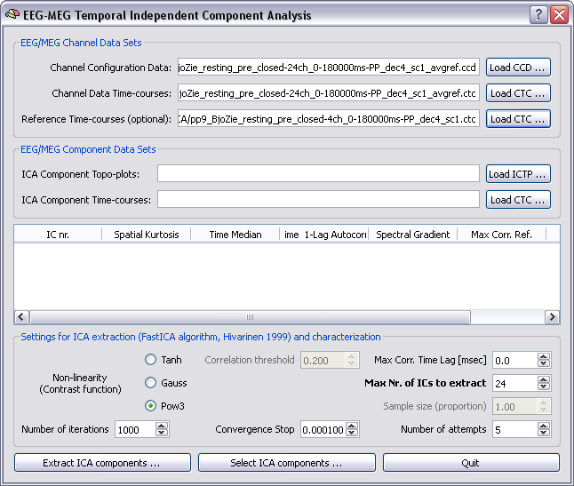
Note: Channel position coordinates must be in the internal BrainVoyager QX coordinate system. If you already registered the current EEG or MEG channel configuration to an head mesh, the spatial transformation from the original (head or device) to the internal coordinate sysyem is stored in the SFH file and channel coordinates can be "copied" from the SFH (/POS) file to the CCD file using the EMEG configutation update plugin, that can be called from the Plugins menu and requires to specify the (pre-registered) SFH file and (for MEG only) the POS file (these are the same files needed for the Forward model calculations).
Algorithm: In this plugin ICA decomposition is achieved by means of the FastICA algorithm invented by Aapo Hivarinen (1999). This algorithm maximises the non-gaussianity of the estimated component time-courses, expressed in term of the negentropy of the component statistical distribution, an information theoretic function defined as the difference between the entropy of a Gaussian random variable with the same mean and variance and the entropy of component itself. Maximizing the non-gaussianity of the components is a fundamental criterion to achieve statistical independece between components. FastICA runs according to a deflation scheme that allows sequentially obtaining the channel weights (unmixing matrix), and hence retrieving the ICs. After each IC estimation, the variance explained by this component is regressed out from the data (decorrelation) and a new IC is estimated. The procedure is stopped when no convergence is possible after a given number of attempts and restarting from random weights, e. g. because the residual signals for all channels only contain gaussian components (i. e. only white noise). From the plugin GUI it is possible to control the principal parameters of the Fastica algorithm, including the specific contrast function (that corresponds to one out of three possible choices for the negentropy approximation with a closed-form non-linear function), the maximum number of ICs and number of attempts for the convergence of each component, the number of iterations of each attempts and the convergence tolerance (convergence stop). More details about how fastICA works and the parameters involved can be found in the scientific papers.
Results: When the estimate of the unmixing weights or coefficients in the linear ICA model is completed, the mixing matrix is computed by means of a pseudo-inversion of the weight matrix. Each column of the mixing matrix, contains the amplitudes of the corresponding component in the recordings. These are stored in an independent component topoplot (ICTP) file and can be displayed in 2D topoplots All component topoplots are stored in independent component topoplot (ICTP) files. Independent component time-courses are stored in a new CTC file, which is formally identical to a channel time-course data set, the only difference being that the channels are conceptually replaced by components. After extraction the ICTP and CTC files are automatically displayed in the GUI and ready for the selection process.
Component time-courses are stored in CTC files, and can be treated similarly to channel time-courses (channels are conceptually replaced by components). After extraction the ICTP and CTC files are automatically displayed in the GUI and ready for the selection process (but can also be loaded independently):
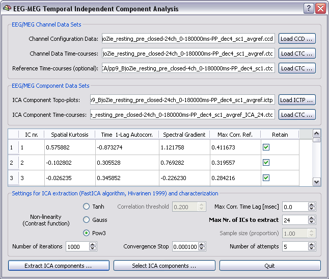
Selection of ICA components requires that both original CTC with channel data and CTC with ICA component data are specified in the dialog. In addition, for each of the ICA components (to be intended in the natural order of extraction) the check box for retaining or not this component should be verified by the user. Upon running the plugin in selection mode, once data are reloaded to working memory, a new data set will reconstructed from the original data set and the estimated components but only the retained components will be considered whereas the other components will be discarded.
ICA Parametric characterization for aiding the selection process. Besides the "Retain" column, useful ICA component spatial and temporal parameters are displayed in the component table for aiding the selection process. These include the spatial kurtosis, the time 1-lag autocorrelation, the spectral gradient and the maximal correlation with reference channels.
Examining the value of the spatial kurtosis often allows to quickly identify a common type of artifact extracted by ICA, characterized by a topoplot with high activity in a single channel and almost no activity otherwise. This is due to short-lasting randomly occurring single-electrode offsets and is reflected in a high kurtosis value in the spatial data, as kurtosis measures the peakedness of data.
There is typically white noise in the acquired data due to hardware aspects. White noise has a close-to-flat frequency power spectrum, as opposed to neurologically relevant EEG components which have a 1/f power spectrum distribution. Residual white noise may remain after general filtering, albeit with a very low contribution. Independent components consisting of white noise can be identified by calculating the 1-lag time autocorrelation and by estimating the slope of the frequency spectrum in terms of the mean spectral gradient. In fact, such artifactual components present relatively low values for both the time 1-lag autocorrelation and the spectral gradient.
In order to facilitate the selection based on these parameters, after calculations for all ICA components, these parameters are scaled to their z-scores over the entire set of components, i. e. the mean and standard deviation of these parameters is calculated over all components and these are respectively subtracted and divided from the original values. As a consequence, provided that enough components are extracted (e. g. >20) absolute values higher than (or close to) 2 point to abnormal component features and therefore, potentially, to artifacts.
When the CTC input with reference channels is provided, the column with the maximal correlation values (not scaled to z-scores) may also gather useful information about artifacts. For instance, to identify artifacts caused by eye blinks (vertical EOG, VEOG) or saccades (horizontal EOG, HEOG), the correlation coefficients of each IC time series with the recorded EOG (typically two VEOG and two HEOG) data channels can be calculated, and the maximum absolute (polarity-free) value is reported in the table. Relatively high values for this parameters may point to artifactual components with prevalent if not exclusive eye blink contribution. Similarly, other types of reference channels such as ECG or EMG channels, when available, may help to identify ICA components with strong or prevalent contribution from cardiac and muscle artifacts. In contrast to EOG, however, the more complex nature of the cardiac and muscle artifacts requires a careful inspection of the components with high correlation values before deciding whether to retain these components or not.
Important note: the ICA parameter table is filled with meaningful values only after extraction of the components, and will remain empty if the ICTP and CTC files are loaded rather estimated in the current run of the plugin. The reason is that two set of ICA components are generally different in order and scale even when these are generated from the same data set.
Examples of typical EEG artifacts detected with ICA
Besides the table with parameters, BrainVoyager offers other visual tools, useful for aiding the selection process. Topoplots, as well continous, event-related average and time-frequency plots (see also channel-level data processing) can be created and visualized from the computed ICTP and CTC data sets before running the selection stage, because the nature of a component can be often identified on the basis of the spatial distribution of the component activities or the phase- or time-locked temporal features with respect to a specific trigger event.
For creating and visualizing topoplots, a specific entry in the EEG-MEG menu is available. For extracting component plots of continous data, time averages and time-frequency dynamics, just load the resulting ICA component CTC (<_ICA_N.ctc>) as any other channel CTC.
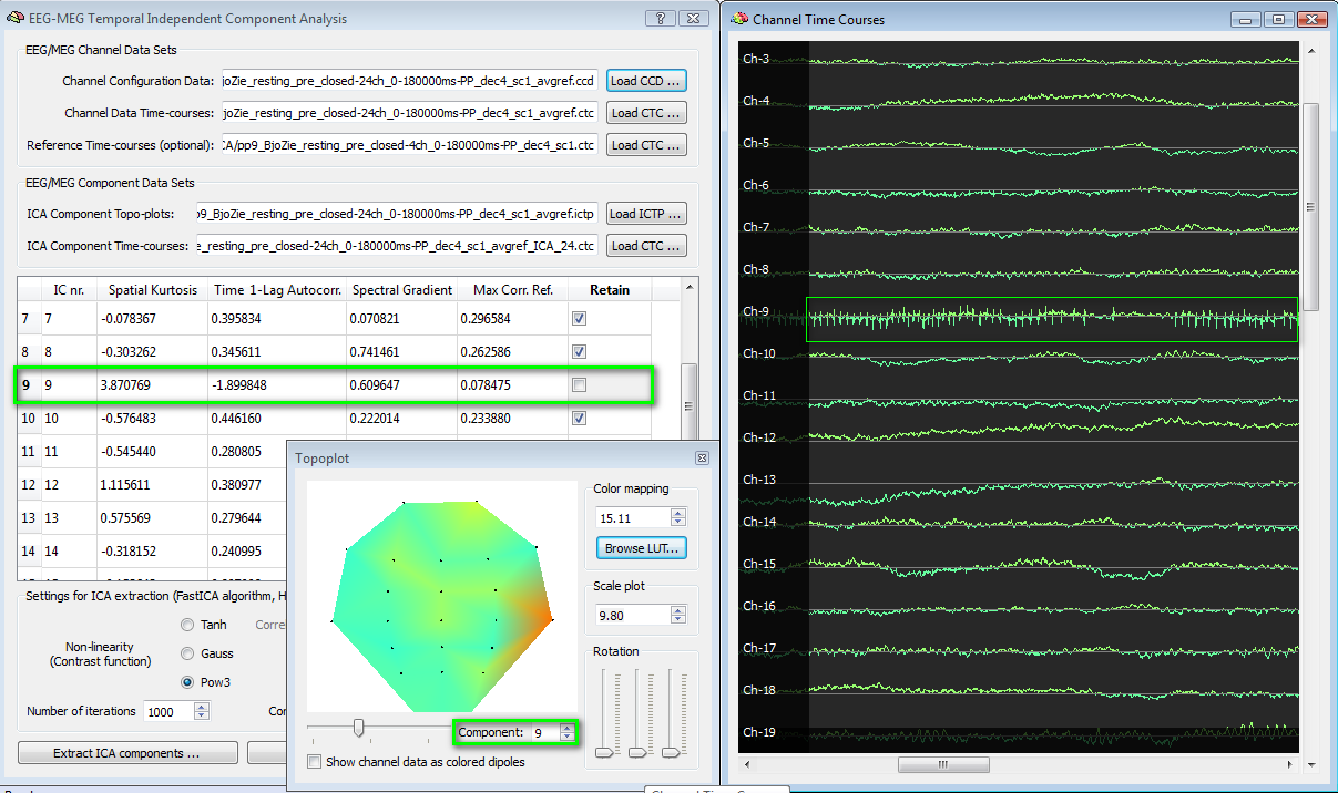
In the example following below, an EEG ICA component (nr. 9) is evaluated in the selection process. The spatial kurtosis exhibits an abnormally high value (>3) and the totoplot confirms the presence of a spatial distribution strongly biased on one single electrode. Finally, by loading the ICA CTC to the EMEG Suite (channel preprocessing tab) it is possible to scroll the entire time-series of all channels and notice, e. g., that signal in channel 9 is not else than a series of spikes, although uncorrelated to eye blinks (max corr ref < 0.1). This component should not be retained.
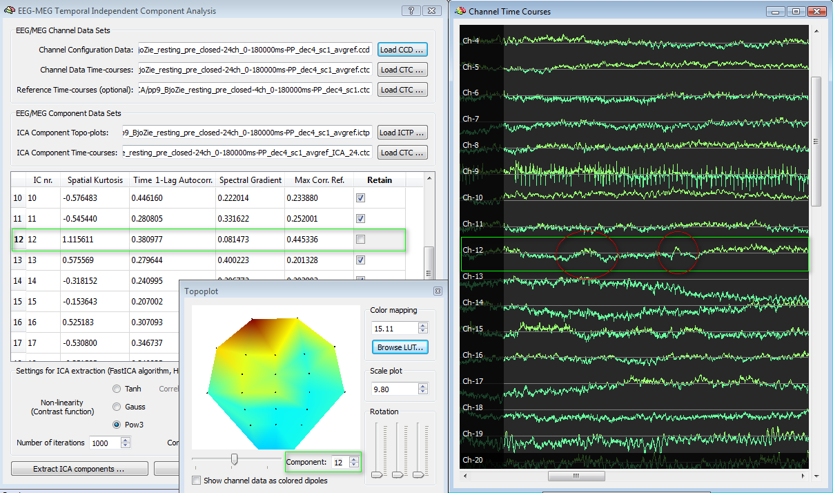
Following the same example, in contrast to IC nr. 9, we may find that IC nr. 12 has not an abnormally high spatial kurtosis (the distribution is biased frontally but certainly less peaked than the IC nr. 9) and more or less normal values of the parameters, but also has a high correlation with the EOG channels (>0.4). Scrolling the plot, it is possible to observe some pulses that clearly point to eye blinks.
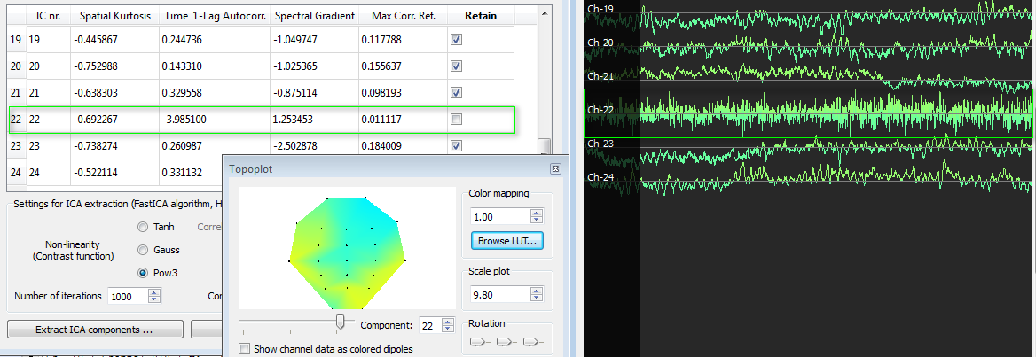
Finally, we also show a white noise component (IC nr. 22). This has abnormally low time 1-lag autocorrelation values (<-3) and the scroll plot confirms the noisy signal of this component. The topoplot shows rather distributed low values and this is also typically of the hardware origin of white noise distributed over all channels.
In sum, the combination of abnormal ICA parameters values with typical visual features may help to identify a certain amount of typical artifacts in EEG (and MEG) data, coming both from techinical and physiological sources.
Note: when there is no converging evidence from numeric and visual features, even if there is suspect of artifacts in a given component, it is good practice to be conservative and initially retain these components. In fact, it is possible that some artifacts might have not been well separated from the useful activity and it might be worth to try and extract new ICA components from the pruned data set. In other words, it makes to sense to run temporal ICA in both extraction and selection modes, more than once, using the reconstructed channel data sets from previous selection run as input for extraction in the subsequent run. In fact, once that some stronger artifacts have been extracted and removed, some more (weaker) artifacts can be more better unmixed from the data and removed in the second iteration.
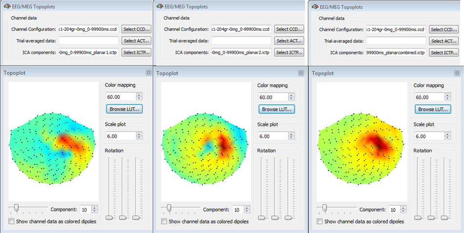
Important note for MEG data sets: Besides the main topoplot data stored in the main ICTP, three additional ICTP files are stored in the same folder, with sufficies <<_planar1.ictp>>, <<_planar2.ictp>>, <<_planarcombined.ictp>>. These files are intended to be used for creating and visualizing topoplotsan only for planar gradiometer MEG configurations (seechapter on file formats and configurations for for more details). Specifically, the <<planar1>> and <<planar2>> ICTP files contains the ICA component topographies where respectively only odd and only even channels are used, whereas the <<planarcombined>> ICTP contains a combination of the two sets of channels according to Pythagora's rule (only positive values). In the case of a planar gradiometer MEG configuration, visualizing the main ICTP file (i. e. the one used for selection and reconstruction of the data from the ICA component) will not provide useful information about the component topographies becuase the two signal types are mixed with each other. An example of three types of topoplots for a planar MEG configuration is shown in the figure below and it is very important to note the complementary information yielded by each topoplot for the same ICA component.
References
Comon P. Independent Component Analysis, a New Concept. Signal Processing 36: 287-314.
Hyvarinen, A., 1999. Fast and robust fixed-point algorithms for independent component analysis. IEEE T Neural Netw. 10, 626-634.
Hyvarinen, A., Oja, E., 2000. Independent component analysis: algorithms and applications. Neural Netw. 13, 411-430.
Hyvrarinen A., Karhunen, J., Oja, E., 2001. Independent Component Analysis. Wiley Eds.
Moran, J.E., Drake, C.L., Tepley, N., 2004. ICA methods for MEG imaging. Neurol. Clin. Neurophysiol. 2004, 72.
Onton J and Makeig S. Information-based modeling of event-related brain dynamics. In: C. Neuper W. Klimesch, Eds., Progress in Brain Dynamics, Elsevier (Amsterdam), 2006.
Vigario, R., Jousmaki, V., Hyvarinen, M., Hari, R., Oja, E., 1998. Independent component analysis for identification of artifacts in magnetoencephalographic recordings. In: Jordan, M.I, Kearns, M.J., Solla, S.A. (Eds.), Advances in Neural Information Processing Systems, vol. 10. MIT Press, Cambridge, pp. 229-235.
Copyright © 2014 Fabrizio Esposito and Rainer Goebel. All rights reserved.