BrainVoyager QX v2.8
Recursive Feature Elimination (RFE)
As discussed in the basic concepts section, it is often desirable to search for discriminative voxels in the whole brain, e.g. if specific (functional) ROIs are not known a priori. In these situations, one would like to find those brain voxels, which are able to discriminate two or more conditions, i.e. one is interested in multivariate brain mapping. One interesting multivariate brain mapping strategy performs a multivariate analysis at each voxel including the responses from voxels in the local neighborhood ("searchlight" approach). Recursive feature elimination (RFE) is another multivariate mapping approach allowing to detect (sparse) discriminative patterns in the brain that is not limited to the local neighborhood of a voxel, i.e. voxels may be spread across the whole brain. The basic principle of RFE is to include initially all voxels of a large region, and to gradually exclude voxels, that do not contribute in discriminating patterns from different classes. Whether a voxel in the current feature set contributes enough to be kept is determined by the weight value of a voxel resulting from training a classifier (e.g. SVM) with the current set of features. in order to increase the likelihood that the "best" voxels are selected, feature elimination progresses gradually and includes cross-validation steps. In each feature elimination step, a small proportion of voxels is discarded until a core set of voxels remains with the highest discriminative power. Note that using SVM to separate "good" from "bad" voxels implements a multivariate feature selection strategy as opposed to univariate feature selection using single-voxel F or t values from a statistical analysis. Nonetheless, an initial feature reduction step using a univariate method might be useful if one wants to restrict RFE to the subset of "active" voxels.
RFE Details
The RFE implemented in BrainVoyager is based on DeMartino et al. (2008). It includes two nested levels of cross-validation to maximize the chance to keep the "best" voxels. At the first level, the training data is partitioned in NF folds and RFE is applied NF times. In each application, one of the folds is put aside for testing generalization performance while the other folds together form the training data for the RFE procedure, i.e. for each of the NF RFE's another "split" of the data is used. When all separate RFE's have been performed, the final generalization performance is determined as the average of the performance across the NF different splits, separately for each reduction level (see below). The final set of voxels (for a specific reduction level) are obtained by merging the voxels with the best weights (highest absolute values) across all splits.
The training data from each first-level split is used for a separate RFE procedure while the fold with the test data is set aside and only used for performance testing. The training data is then partitioned again in L sub-folds and a SVM is trained on L splits in order to obtain robust weight rankings for feature elimination. A voxel's ranking score is obtained by averaging the weights of that voxel across the different second-level splits. The absolute values of these scores are then ranked and the voxels with the lowest ranks are removed. The "surviving" voxels are then used for the next RFE iteration, which starts again with (a new) partitioning of the data in L folds. The whole procedure is repeated R times until a desired number of voxels has been reached. As described above, the RFE level producing the highest generalization performance across all first-level splits is finally selected and the level's set of voxels is determined by merging the best voxels of the respective first-level splits.
Application
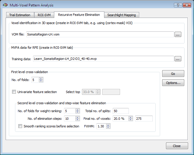
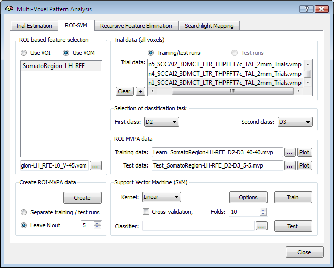
The figure above shows the Recursive Feature Elimination tab of the Multi-Voxel Pattern Analysis dialog. To perform RFE, two input sources are required, a VOM file and a MVP file. As described earlier, a VOM is similar to a VOI with the exception that voxels are stored in the resolution of functional data (VTCs/VMPs) instead of the resolution of the "hosting" anatomy (VMR); furthermore a VOM may contain for each voxel a floating-point value (e.g. a statistical map value or a SVM weight). The VOM file can be created from a VOI in the ROI-SVM tab or using the Create VOM dialog (Options > Create VOI Map menu item). Starting from a VOM (derived from a VOI) allows to determine the size of the brain region to be used for recursive feature elimination. While RFE can be applied to the whole brain, it is often more appropriate to select a large interesting region, such as the visual cortex or the frontal lobe. When such restrictions are not desired, it is best to convert a cortex mask VOI to a VOM. The "..." selection button on the right side of the VOM file text field to select the desired brain region.
The second input needed for RFE is a MVP file containing the training data for the initial (full) set of voxels corresponding to those in the selected VOM file. The easiest way to get both the VOM and the desired MVP file is to use the ROI-SVM tab, which allows to extract estimated BOLD responses for any region of interest as described in section Applying SVMs to ROIs. If trial estimates for the desired data are not yet available, you must first estimate them from a set of selected VTC files (Trial Estimation tab) resulting in a set of VMP files containing the trial estimates per voxel. When clicking the Create button in the Create ROI-MVPA data field of the ROI-SVM tab, a specified VOI is first converted in a VOM to get the voxels in native resolution. The VOM voxels are then used to extract the trial responses from the VMP files. The result is stored in a MVP file in form of a "trial responses x voxels" matrix (see plots below). Note that a VOM file forms an important link between the voxels in the MVP matrix and the location of the voxels in the brain: the i'th entry in a MVP file contains trial estimates but no voxel coordinates while the i'th entry in a VOM file contains the voxel's x, y and z coordinates. Because of this important link, the program creates a MVP file and a VOM file with the same name when extracting trial estimates from VMP files. In the used somatosensory example data, the VOM name (and original VOI name) is "SomatoRegion-LH" and this name appears also in the selected MVP file (see above) indicating that both files refer to the same voxels.
With the input specified, the RFE procedure can be started by clicking the GO button. If desired, the RFE procedure that will be executed can be modified before by setting some options. The number of first-level folds (NF) can be specified using the No. of folds spin box in the First level cross-validation field, which is set to "5" as default. While RFE implements a multivariate feature selection strategy, it may be useful to restrict the number of voxels to some extent using a univariate strategy. In order to add univariate selection prior to RFE (performed for each first-level split), the Univariate feature selection option can be turned on. By changing the value in the Select top percent spin box, the desired percentage of "surviving voxels" can be specified. Note that when the percentage value is changed, the respective absolute number of remaining voxels after univariate feature selection is shown in the the text field on the right side of the Select top percent spin box.
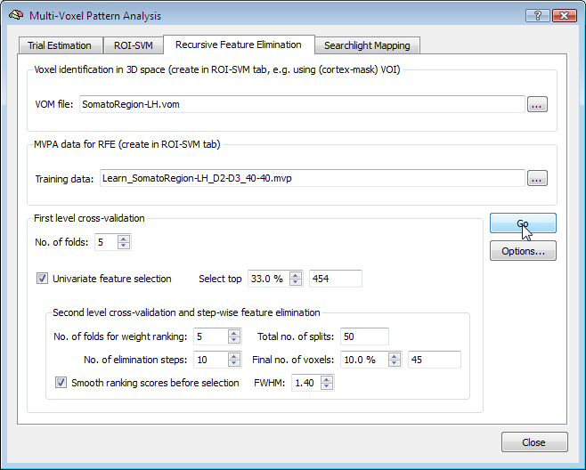
The Second-level cross-validation and stepwise feature elimination field is visually nested within the First level cross-validation field indicating that the RFE procedure is performed for each first-level split. At each RFE level (see below), the data is partitioned again in a number of folds (Nx), which can be adjusted using the No. of folds for weight ranking spin box. For each of the created splits, a supprt vector machine is trained and the weights are ranked according to their absolute value. The voxels with the highest weights across all splits are selected. The voxels are, however, not reduced to the final number in one step, but RFE proceeds stepwise resulting in several "RFE levels". The number of RFE levels can be specified by changing the No. of elimination steps spin box (default: 10). Using such a stepwise procedure should help, like the cross-validation approach, to increase the robustness in finding the "best" voxels. The percentage of target voxels, which should remain after running through all RFE levels can be specified in the Final no. of voxels spin box. The text field on the right side of this spin box shows the corresponding absolute number of voxels. Note that If the univariate selection option is enabled, the specified percentage is applied relative to the number of voxels filtered by univariate feature elimination.
The Smooth ranking scores before selection option allows to slightly smooth spatially the obtained ranking values prior to selection. This step will introduce a bias towards favoring spatially clustered regions over isolated voxels. In some applications, this smoothing step proved beneficial if the width of the filter is small, e.g. with a full-width at half maximum (FWHM) of 1.2-1.5. In the example above the value in the FWHM spin box has been changed from the default value "1.3" to "1.4".
After running RFE, you will see a plot showing the average generalization performance assessed with the separated test data sets for each RFE level (see below). While not always the case, the generalization performance often increases while decreasing the number of voxels. Note that because of random generation of folds, you will not get exactly the same results (nor exactly the same voxels) if you re-run the procedure with the same settings.
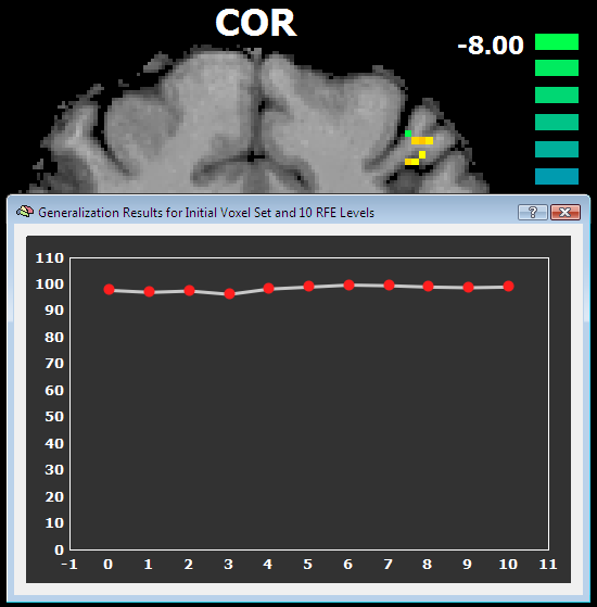
Besides the generalization performance plot, the RFE will also show the resulting voxels and associated weights by automatically visualizing the resulting VOM as a volume map (VMP). The figure above shows a slice to the somatosensory cortex showing some of the 45 remaining voxels. The figure below shows the effect of rank smoothing on voxel selection. For the D2/D4 classification task, the left pane shows the SVM weights for a sagittal slice with the original ("full") voxel set and after RFE (middle and right pane) with a final number of 68 voxels (no univariate selection).
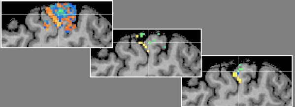
The middle panel shows the result when smoothing was turned off, while the panel on the right side shows the result when smoothing was used with a FWHM value of 1.4. While already visible with the full voxel set, RFE seem to have indeed found voxels separating the two digits D2 and D4.
Visualization of weights across selected voxels
The ROI-SVM tab provides the possibility to extract training data from trial estimation VMP files using a VOM instead of a VOI file (see snapshot below). To specify a VOM file, the Use VOM option must be selected in the ROI-based feature selection field before using the "..." selection button. This option allows to visualize the trial response data for the reduced voxel set of the final RFE level.
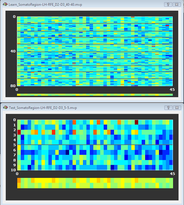
The top panel in the figure below shows the D2/D4 training data for the 45 voxels remaining after RFE, which can be compared to the plot shown in the ROI-SVM section showing the same training and test data for the original set of voxels (1378). As explained in the ROI-SVM section, the black lines separate the trials of the D2 and D4 class. The two "lines" at the bottom of the plot show an average of the voxels' responses separately for each class. As compared to the full voxel plot, it becomes evident that the voxels selected are indeed "good" voxels since they often show clearly different values for the two classes.
References
De Martino F, Valente G, Staeren N, Ashburner J, Goebel R., Formisano E. (2008). Combining multivariate voxel selection and support vector machines for mapping and classification of fMRI spatial patterns. NeuroImage, 43, 44-48.
Copyright © 2014 Rainer Goebel. All rights reserved.