BrainVoyager QX v2.8
Visualization Of Depth Grids and Sampled Data
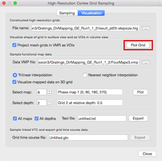
When the grid sampling process has completed, the program switches automatically to the Visualization tab (see snapshot above). The File name text entry in the High-resolution grid file field will display the file name of the produced (".hrg" or ".txt") grid file that is loaded automatically and available for visualization. In case you have previously stored grid files that you want to use for visualization, you do not need to rerun the sampling process: simply load a stored grid file using the Browse ("...") button on the right side of the File name text field.
Grid Visualization
In order to visualize the grid, click the Plot Grid button (see above). The grid will be shown as a series of horizontal and vertical lines (rows and columns of the grids) in the surface rendering window; if no surface window is attached to the VMR, it will be created automatically; it is, hoever, recommended to load a matching reconstructed mesh for advanced visualizations (see below). The horizontal and vertical lines belonging to the same grid (same relative depth level) are shown in the same color and different grids will be shown with different default colors (see snapshot below).
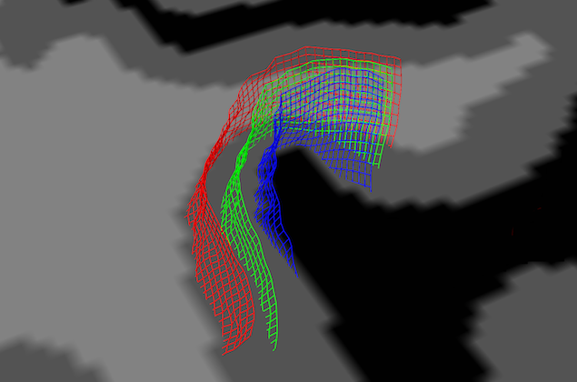
In order to see the grid lines with respect to neighboring anatomical information, turn on texture slicing by clicking on one of the slicing icons. In the snapshot above, the Tra Slicing Mode icon has been clicked and the appearing axial slice has been positioned at a level that intersects the grid lines. This helps to view the different depth levels sampled by the grids. As stated above, the grids will be oriented along the specified VOI or, if the 3D reference point approach is used, they will be roughly centered around the chosen 3D coordinates in the VMR data. Note, however, that the axial slice is probably left-right flipped with respect to the VMR data since the surface visualization always attempts to depict the data in neurological convention (right-is-right) independent of the convention used for the VMR data set (which is usually radiological convention, left-is-right).
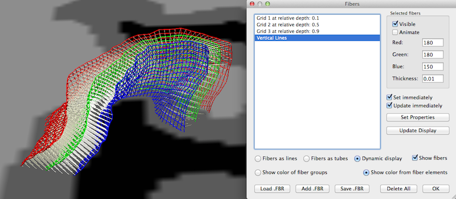
Note that the grid lines are drawn using the fiber visualization tools originally developed for DTI fiber tracking visualization. You may, thus, apply any visualization option available for fibers also for the grid lines using the Fibers dialog (see snapshot above), e.g. you may change the thickness of the grid lines and visualize grid lines as tubes instead of lines. For advanced visualizations like animations and slice-restricted visualization (see below) the Dynamic display option needs to be selected (see snapshot above). Since the names of the grids contain information about the respective depth level, you may also use the Visible option in the Selected fibers field to show or hide specific depth level grids. Note that the created visualization not only shows the grid lines but also the streamlines connecting homologue grid points across different depth levels. To hide these lines, turn on/off the Visible option after selecting the entry "Vertical Lines" in the Fibers list.
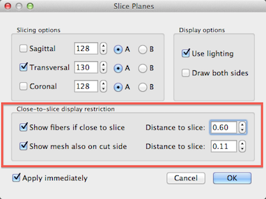
In order to improve visual inspection of how the grids follow the cortical ribbon at different depth levels, it is possible to restrict drawing of the grid lines to a specified distance from the current slicing level. In order to activate this option, click the Texture Slicing item in the Meshes menu to invoke the Slice Planes dialog (see screenshot above). To restrict grid (fiber) display in relation to the current slice position, turn on the Show fibers if close to slice option in the Close-to-slice display restriction field (see above). Use the Distance to slice spin box to adjust the distance from the current slice beyond which you do not want to see the grid rendering. Note that this option only has an effect if the Dynamic display option is checked in the Fibers dialog. Another similar option in this dialog allows to show a sliced mesh "through" the cut on the other side. This may also be helpful to visualize how one or more cortex meshes run along the cortex at different relative depth levels. This visualization option may be turned on by checking the Show mesh also on cut side option. As with the grid (fiber) display, you may specify a distance value by adjusting the value in the Distance to slice spin box on the right side of the Show mesh also on cut side option.
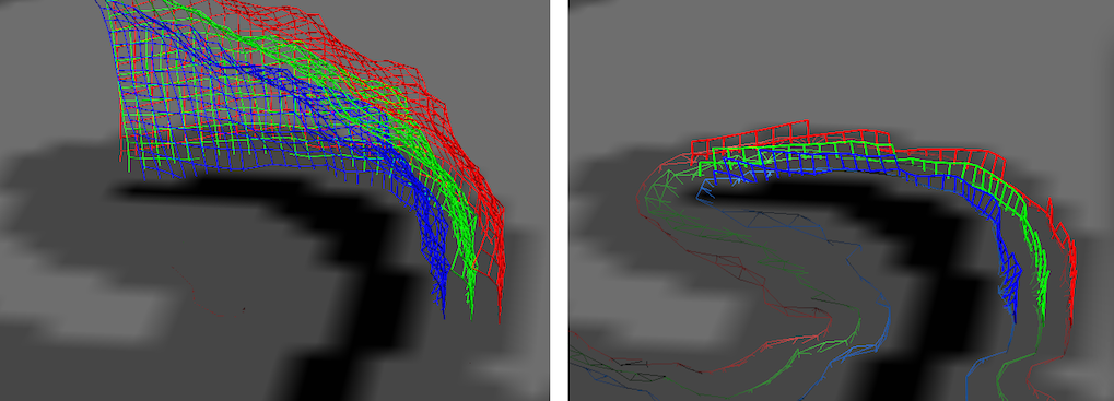
In the snapshot above, the left side shows the initial display of the grid lines while the right side shows the display after turning on both slice restrictions options. Since this distance setting is in effect when slicing the mesh, it allows easy inspection of the quality of reconstructed relative cortical depth levels.
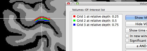
In case that the Project mesh grids in VMR as VOIs option is turned on (default) in the Visualization tab when clicking the Plot Grid button, the created grids will be also visualized as VOIs in the VMR view (see snapshot above and below showing different grid sampling examples).
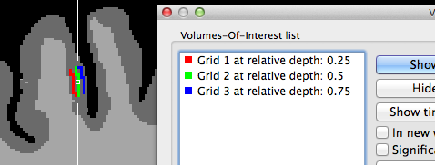
The two snapshots above indicate that the grids are created roughly symmetrical around the chosen reference point in the horizontal and vertical direction (the 3D reference point has been used for these examples). The horizontal extent is larger than the vertical one since the specified number of grid columns was set to 40 while the number of rows was set to 20 in this example. The snapshot depicts also part of the Volumes-Of-Interest dialog showing the VOIs that have been automatically created as the result of projecting the grid lines into the VMR; note that the VOI names indicate the color and depth level belonging to a specific VOI; you may use this information to visualize specific depth levels or to turn off the "Vertical Lines" VOI since that, due to resolution limitations in voxel space, will hide the individual grid VOIs. The grids are better visible if the VOIs are rendered opaque; this can be achieved either by using the Shift-Ctrl/Cmd-Cursor-Up/Down key combination or by setting the Value spin box in the VOI transparency field of the VOI Analysis Options dialog to 1.0. Note that an alternative approach is available to create depth VOIs, which should be used if separate (non-overlapping) voxels should be included in the sub-VOIs.
Mapping Functional Data
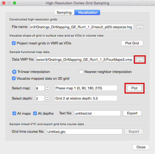
The main purpose of creating the grids is to sample functional data in a topographically precise way at different cortex depth levels. The middle section of the Visualization tab of the High-Resolution Cortex Grid Sampling dialog (see snapshot above) allows to load a (native-resolution) volume map from which map data can be extracted and visualized on the created grids. It may be that the Data VMP file text box in the Sample functional map data field shows the name of a previously used volume map, e.g. the cortical thickness map used for grid sampling. In order to load a different VMP file containing the desired functional data, use the Browse ("...") button on the right side of the Data VMP file text box (see snapshot above); you may also use the Volume Maps dialog to load map files. In case that the loaded VMP file contains several sub-maps, you can select a specific map for data extraction using the Select map spin box; the name of the selected sub-map will be displayed in the text box on the right side of the Select map spin box ("Phase map 1" in the example above). Before being able to map functional data on grids, a grid file (.hrg or .txt) needs to be loaded (or created). If grids are available, the Select depth spin box can be used to select a desired grid at a specific depth level that will be used to read the functional data; the name of the selected grid will be displayed in the text box on the right side of the Select depth spin box.
To start the data sampling from the specified grid, click the Plot button in the Sample functional map data field. As default, grid points will sample the functional (map) data using trilinear interpolation as indicated by the checked Trilinear interpolation option. In case you want to sample the data using nearest neighbor interpolation, click the Nearest neighbor interpolation option before clicking the Plot button. In order to sample more than one depth level, simply repeat this step, each time selecting a different depth level grid for the same or different volume map. In the example case shown above in the dialog, the functional map 8 ("Phase map 1 (0, 90, 180, 270)") and the second grid ("Grid 2 at telative depth: 0.5") have been chosen.
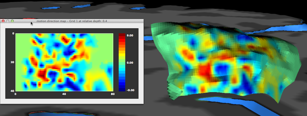
The result of the functional sampling of the selected grid and the selected sub-map will be visualized as an image in a matrix plot: each pixel in the image is filled with the value sampled by the corresponding point in the grid. The sampled values are visualized using a default look-up table that can be changed if desired (see below). Besides the 2D image plot, the same data is also visualized directly on the 3D grid (in case that the Visualize mapped data on 3D grid option has been selected), i.e. precisely at the 3D points (vertices) defining the grid. This is the same kind of visualization as when a surface map is projected on a cortex mesh but here the data is sampled at very high resolution potentially revealing functional clusters (cortical columns) at different cortex depth levels within specialized areas (the example above depicts axes-of-motion columns in area hMT, see Zimmerman et al., 2011).
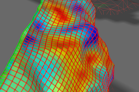
Note that one can also combine display of the grid lines (fibers) with mapped functional data as shown in the screenshot above.
In order to change settings of the image shown in Matrix Plot dialog, click somwhere within the dialog to launch the Matrix Plot Options dialog (see below). In this dialog, you may change the maximum value in the Scale value spin box to scale the data differently - as default the absolute maximum value is used to scale the map values to the color look-up table (LUT). You may also load a different LUT as has been done in the snapshot below using the Load LUT button and selecting, e.g. the "hsv_inv.olt" or "angle_hsv_v1.olt" file. Note that the Matrix Plot Options dialog can also be used to obtain a numerical representation of the sampled values by clicking the Data Table button; from the appearing Matrix Data Table dialog, you can also save the sampled grid values to disk for further use.
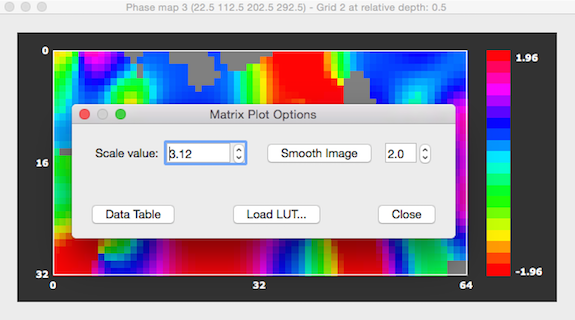
It is also possible to smooth the sampled functional data with a Gaussian 2D kernel by clicking the Smooth Image button. The full-width at half maximum (FWHM) value of the kernel can be changed by using the Smooth Image spin box on the right side of the button. Besides increasing the FWHM value, the amoutn of smoothing can also be changed by clicking the Smooth Image button repeatedly. Smoothing is performed using bilinear interpolation. Pixels that have a value of exactly 0.0 are treated as missing values and are not changed and not included in the smoothing process of other voxels. Furthermore, if the matrix plotter contains angle (phase) map values between -PI and +PI, smoothing will respect the circular nature of this map type.
Exporting Map and Time Course Data
When sampling functional data, the sampled map values will not only be shown in the matrix plotter (from where it can be saved via the Data Table button) but also printed in BrainVoyager's Log pane. Furthermore, the sampled data can be exported in a text file for further processing (e.g. in Matlab) using the Export button in the Sample functional map data field. The triggered export function can be used to quickly get sampled map data for all depth levels by turning on (default) the All depths option prior to using the Export button; it is also possible to save sampled map values not only from the map selected in the Select map field but for all maps in the loaded VMP data in case that the All maps option has been turned on (default). The number of maps and grids is not specified in the header but they can be identified by their stored names. Also the dimensions of the grids are not stored at present but you can derive them from the corresponding exported grid (text) file (see format description in previous topic) since each sampled map value corresponds to a specific grid point in the saved grid file. The format for N grids and M maps of the stored text file is as follows:
GridDataFileVersion: f [only file version "1" supported until now]
[Loop m: No. of maps, all maps or selected one depending on chosen option]
    Map-m: MapName [name of map in parentheses]
    [Loop d: No. of grids, all grids or selected one depending on chosen option]
    Grid-At-Depth-d: GridName [name of grid in parentheses]
        [Loop y: No. of grid rows]
            [Loop x: No. of grid columns]
                sampled map value from map m at grid point x, y, d
            [Loop x end]
        [Loop y end]
    [Loop d end]
[Loop m end]
Besides map data, the Export button in the Sample linked VTC and export grid time course data field allows to sample and export time course data for each grid point from a currently linked VTC file. In case that no VTC file is available, the Export button is disabled (greyed out). The time course data is stored in a grid time course (.gtc) file (little endian byte order). The .gtc file has a simple header that stores the dimensions of the data; after the header, the sampled time course data contains one 4-byte float value for each time point of each grid point:
f [4-byte integer, only value 1 at present]
D [4-byte integer, number of grids]
Y [4 byte integer, number of rows in single grid]
X [4 byte integer, number of columns in single grid]
T [4 byte integer, number of time points per grid point, extracted from linked VTC]
[Loop d: No. of grids]
    [Loop y: No. of grid rows]
        [Loop x: No. of grid columns]
            [Loop t: No. of time points]
                 value at time point t for grid point x, y, d [4-byte float]
            [Loop t end]
        [Loop x end]
    [Loop y end]
[Loop d end]
If you have any questions concerning the exported file formats, please send an email to support at brainvoyager dot com.
References
Zimmermann, J., Goebel, R., De Martino, F., van de Moortele, P.F., Feinberg, D., Adriany, G., Chaimov, D., Shmuel, A., Ugurbil, K., Yacoub, E. (2011). Mapping the organization of axis of motion selective features in human area MT using high-field fMRI. PLoS One, 6 e28716.
De Martino F., Zimmermann J., Muckli L., Ugurbil K., Yacoub E., Goebel R. (2013). Cortical Depth Dependent Functional Responses in Humans at 7T: Improved Specificity with 3D GRASE. PLoS One, 8, e60514.
Copyright © 2014 Rainer Goebel. All rights reserved.