BrainVoyager QX v2.8
Segmentation of the WM-GM Boundary
After performing the preparatory steps for advanced segmentation, the tools available in the WM-GM Border tab of the Advanced Segmentation Tools dialog (see snapshot below) can be used to segment the white / grey matter boundary.
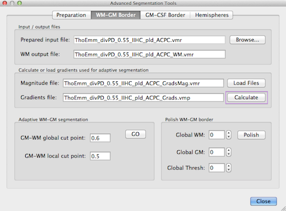
The current VMR file name is shown in the Prepared input file text box. If you would like to process another prepared file, you can use the Browse button on the right side of the text box. The WM output file text box shows the name under which the resulting file of the subsequent WM-GM segmentation steps will be saved to disk. The "_WM" extension indicates that the resulting file will contain an explicit labelling of white matter voxels.
The most important function of this tab is an adaptive region growing step, which uses two sources of information to separate white from grey matter voxels. One source are locally computed intensity histograms (see below) and one source consists in gradient information. The latter information source needs to be calculated before starting the adaptive segmentation process. To compute the gradient information, click the Calculate button in the Calculate or load gradients used for adaptive segmentation field. If you have previously computed these files, you may also reload them by clicking the Load Files button. After calculating the gradients, the dialog will show the names of two files containing relevant information (see snapshot above).
The VMR file shown in the Magnitude file text box contains voxels along boundaries of maximum gradient information. These boundaries typically run along the white / grey matter boundary as well as along the grey matter / CSF boundary. It is kept in memory as a secondary VMR and can be inspected by using the F8 button to toggle between the primary and secondary data set. While the maximum gradient VMR data set helps to identify boundaries, it does not contain directional (gradient) information. The VMR file shown in the Gradients file text box is a VMP file containing three sub volume maps. The three maps contain for each voxel the x, y, and z component of the voxel's gradient vector, which is used to determine which side of the gradient magnitude contour lies inside or outside of white (or grey) matter. The gradient maps constitute the basic data that is also used to calculate magnitude values by computing the length of a voxel's gradient vector as defined by the three voxel component values. Note that the gradients VMP file is usually very large (ca. 350 MB) so that loading and saving that file may last a few seconds.
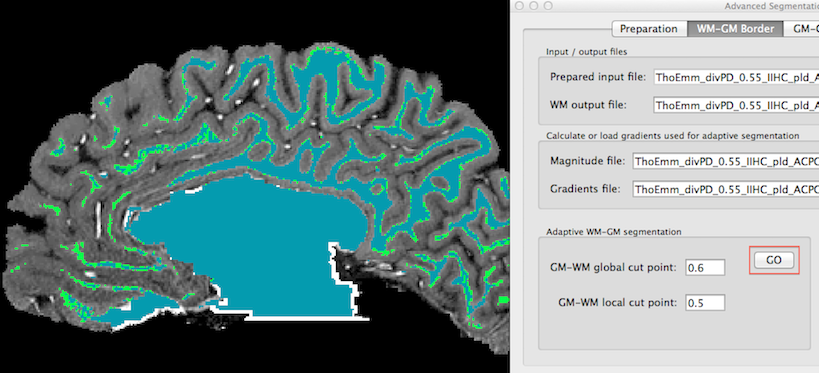
The main function of this tab, adaptive WM segmentation, is launched by clicking the GO button in the Adaptive WM-GM segmentation field (see right side in snapshot above). The adaptive segmentation procedure starts by globally analyzing the distribution of intensity values to find an initial threshold to segment white and grey matter. The threshold is determined as a value between the global white matter and grey matter peak. The GM-WM global cut point value can be used to shift the threshold more towards the white or the grey matter peak. A value of 0.5 would use the intensity value in the middle of the two peaks. While the default value is normally working fine, it is possible to optimize segmentation results by changing this value. Using a threshold closer to the WM peak is recommended since the segmentation is not only based on this value but also on an analysis of the local histogram information around a voxel. During processing, a plot of the global histogram (averaged from several local histograms) is shown.
The estimated WM and GM peaks may differ across space measured by calculating local intensity histograms in many sub-cubes of the data. The WM-GM threshold for each local histogram can be biased in a similar way as the global value by entering a separate value in the GM-WM local cut point text box. For the example data, this value has been kept at the default (0.5).
After some processing time, the result of the adaptive segmentation is shown. The blue colored voxels show those resulting from the fixed global threshold and the green color shows voxels that have been additionally labelled by the local histogram analysis (see snapshot above, left side). The benefit of adaptive segmentation is the inclusion of thin white matter regions, which are sometimes missed by a global segmentation process.
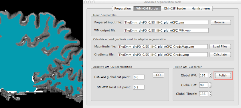
The estimated white / grey matter border is usually somewhat noisy after the adaptive segmentation step. In order to estimate a more smooth WM / GM contour, the program "polishes" the boundary by calculating a magnitude map based on computed gradient maps. This operates in a similar way as described above, but the border to calculate gradients is not based on the original intensity values but on the binary segmentation result (blue voxels -> foreground, other voxels -> background). The polishing step is started by clicking the Polish button in the Polish WM-GM border field. The snapshot above shows the resulting white matter segmentation (blue color) for one sagittal slice.
In some regions with low contrast the white matter may extent to grey matter up to the CSF boundary. Since BrainVoyager QX 2.8 this is at least partially prevented by limiting the spread of white matter voxels, i.e. they are not allowed to be closer to CSF voxels than 1.5 mm.
After completion of the WM-GM step, the data set is ready for grey matter / CSF segmentation.
Copyright © 2014 Rainer Goebel. All rights reserved.