BrainVoyager QX v2.8
Basic Statistical Principles
In this section, basic principles of statistical analysis are described focusing on the time course measured at a single voxel.
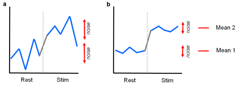
In the figure above two fMRI time courses are shown, which have been obtained from two different voxels in an experiment with two conditions, a control condition ("Rest") and a main condition ("Stim"). Each condition has been measured several times. Note that in a real experiment, one would not just present the control and main condition only once, but one would design several "on-off" cycles in order to be able to separate task-related responses from potential low-frequency drifts (see Preprocessing of functional data).
From Subtraction to Statistical Comparison
How can one assess whether the response values are higher in the main condition than in the control condition? One approach consists in subtracting the mean value of the "Rest" condition, X1, from the mean value of the "Stim" condition, X2: d = X2-X1. Note that one would obtain the same mean values and, thus, the same difference in cases a) and b). Despite the fact that the means are identical in both cases, the difference in case b) seems to be more "trustworthy" than the difference in case a) because the measured values vary less in case b) than in case a). Statistical data analysis goes beyond simple subtraction by taking into account the amount of variability of the measured data points. Statistical analysis essentially asks how likely it is to obtain a certain effect if there would be only noise fluctuations. This is formalized by the null hypothesis stating that there is no effect, i.e. no difference between conditions. In the case of comparing the two means μ1 and μ2, the null hypothesis can be formulated as: H0: μ1 = μ2. Assuming the null hypothesis, it can be calculated how likely it is that an observed effect would have occurred simply by chance. This requires knowledge about the amount of noise fluctuations which can be estimated from the data. By incorporating the variability of measurements, statistical data analysis allows to estimate the uncertainty of effects (e.g. mean differences) in data samples. If an effect is so large that it is very unlikely that it has occurred simply by chance (e.g. the probability is less than p = 0.05), one rejects the null hypothesis and accepts the alternative hypothesis stating that there exists a true effect. Note that the decision to accept or reject the null hypothesis is based on a probability value which has been accepted by the scientific community (p < 0.05). A statistical analysis, thus, does not prove the existence of an effect, it only suggests "to believe in an effect" if it is very unlikely that the observed effect has occurred by chance. Note that a probability of p = 0.05 means that if we would repeat the experiment 100 times we would accept the alternative hypothesis in about 5 cases although there would be no real effect. Since the chosen probability value thus reflects the likelihood of wrongly rejecting the null hypothesis, it is also called error probability.
Statistical Comparison of Means: t Test
The uncertainty of an effect is estimated by calculating the variance of the noise fluctuations from the data. For the case of comparing two mean values, the observed difference of the means is related to the variability of that difference resulting in a t statistic:

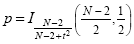
The numerator contains the calculated mean difference while the denominator contains the estimate of the expected variability, the standard error of the mean difference. Estimation of the standard error involves pooling of the variances obtained within both conditions. Since we observe a high variability in case a) in the example data (see figure above), we will obtain a small t value. Due to the small variability of the data points in b), we will obtain a larger t value in this case (see figure above). The higher the t value, the less likely it is that the observed mean difference is just the result of noise fluctuations. It is obvious that measurement of many data points allows a more robust estimation of this probability than the measurement of only a few data points. The error probability p can be calculated exactly from the obtained t value using the incomplete beta function Ix(a,b) and the number of measured data points N:
If the computed error probability falls below the standard value (p < 0.05), the alternative hypothesis is accepted stating that the observed mean difference exists in the population from which the data points have been drawn (i.e. measured). In that case, one also says that the two means differ significantly. Assuming that in our example the obtained p value falls below 0.05 in case b) but not in case a), we would only infer for brain area 2 that the "Stim" condition differs significantly from the "Rest" condition.
Correlation Analysis
The described mean comparison method is not the ideal approach to compare responses between different conditions since this approach is unable to capture the gradual profile of fMRI responses. As long as the temporal resolution is low (volume-TR > 4 seconds), the mean of different conditions can be calculated easily because transitions of expected responses from different conditions occur within a single time point. If the temporal resolution is high (e.g., 2 seconds), the expected fMRI responses change gradually from one condition to the next due to the sluggishness of the hemodynamic response. In this case, time points cannot be assigned easily to different conditions. Without special treatment, the mean response can no longer be easily computed for each condition. As a consequence, the statistical power to detect mean differences may be substantially reduced, especially for short blocks and events. This problem does not occur when correlation analysis is used since this method allows explicitly incorporating the gradual increase and decrease of the expected BOLD signal. A predicted gradual time courses is used as the reference function in a correlation analysis. At each voxel, the time course of the reference function is compared with the time course of the measured data by calculation of a correlation coefficient r, indicating the strength of covariation:
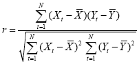
Index t runs over time points (t for "time") identifying pairs of temporally corresponding values from the reference (Xt) and data (Yt) time courses. In the numerator the mean of the reference and data time course is subtracted from the respective value of each data pair and the two differences are multiplied. The resulting value is the sum of these cross products, which will be high if the two time courses covary, i.e. if the values of a pair are both often above or below their respective mean. The term in the denominator normalizes the covariation term in the numerator so that the correlation coefficient lies in a range of -1 and +1. A value of +1 indicates that the reference time course and the data time course go up and down in exactly the same way, while a value of -1 indicates that the two time courses run in opposite direction. A correlation value close to 0 indicates that the two time courses do not covary, i.e. the value in one time course cannot be used to predict the corresponding value in the other time course.
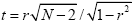
While the statistical principles are the same in correlation analysis as described for mean comparisons, the null hypothesis now corresponds to the statement that the population correlation coefficient rho equals zero (H0: ρ = 0). By including the number of data points N, the error probability can be computed assessing how likely it is that an observed correlation coefficient would occur solely due to noise fluctuations in the signal time course. If this probability falls below 0.05, the alternative hypothesis is accepted stating that there is indeed significant covariation between the reference function and the data time course. Since the reference function is the result of a model assuming different response strengths in the two conditions (e.g. "Rest" and "Stim"), a significant correlation coefficient indicates that the two conditions lead indeed to different mean activation levels in the respective voxel. The statistical assessment can be performed also by converting an observed r value into a corresponding t value:
The described t test and correlation analysis are limited to the comparison of two conditions. The General Linear Model extends these approaches to the case of multiple conditions.
Copyright © 2014 Rainer Goebel. All rights reserved.