BrainVoyager QX v2.8
Inclusion of Statistical Data Sets
For brain imaging it is important to integrate volume maps in the volume rendering process, e.g. to allow visualization of statistical results showing activated brain regions. Any volume map that is overlaid on the current VMR before starting the volume renderer will be available for display. You may open the Volume Maps dialog in order to view the currently available and overlaid (checked) volume maps.
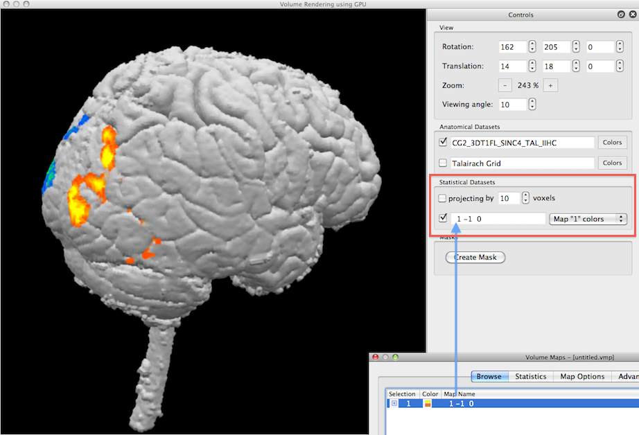
In the example snapshot above, the Volume Maps dialog shown on the right lower side lists one checked volume map that results from a simple statistical contrast; after starting the volume renderer, that map is available for visualization in the Statistical Datasets field (see red rectangle). Since the available map is checked (see blue arrow), the Render View shows the current volume together with the statistical map. Note that the maps imported from the Volume Maps dialog are incorporated in volume rendering with their respective color definitions, statistical threshold and cluster-size threshold.
Since the rendered volume is the result of a brain extraction process, the map is only visible at the outer grey matter border. Such a view will, of course, hide activity that is inside the brain. There are several possibilities to exhibit activity inside the brain, including cutting, projection and transparency.
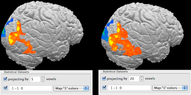
The projection option allows to project activity inside a volume (e.g. a rendered brain) to the visible border of the rendered volume. Technically, rays sent from an image plane inside the volume are not stopped (as usual) when they reach a certain intensity (rendered as visible border) but they are allowed to "look inside" by traveling a specified number of voxels further along the ray direction; if a ray "finds" map data, it will be visualized and appears to be located at the rendered border of the volume, i.e. the inside map values are "projected out" to the visible border; this process depends on the current viewpoint (direction of rays). The projection method is turned off as default and can be used by checking the Projecting by option in the Statistical Datasets field. The number of voxels that the rays move inside the volume after hitting the rendered boundary is specified in the Voxels spin box. In the example snapshots above, the projection method has been used for the map shown before without projection now using projection with 5 (left side) and 20 (right side) voxels.
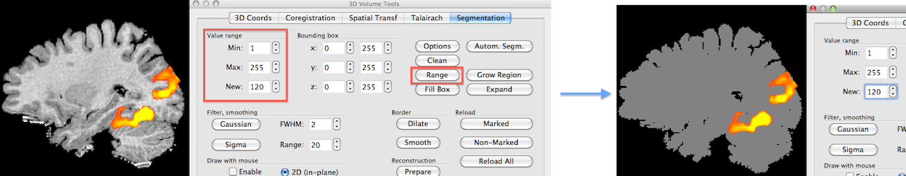
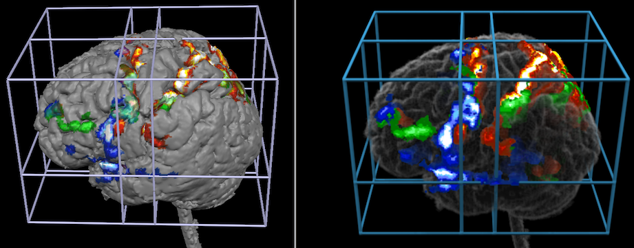
Using transparency is another approach to visualize activity inside the brain. As shown in the previous topic, colors can be defined for volumes (even different colors for specified intensity ranges) including an opacity value. In order to obtain "glass brain" like renderings, it is helpful to use segmented brains as input for volume rendering that have all intensities set to the same value since this will avoid that anatomical structures "interfere" with highlighting volume maps. The snapshots above show how to set intensity values to a single value using the spin boxes in the Value range field in the Segmentation tab of the 3D Volume Tools dialog; to include all possible intensities in a range, the Min intensity value must be set to "1" and the Max intensity value must be set to "255"; the new value can be set to any desired non-zero value but to actually see the result the value should be "100" or higher (in the example, a value of "120" is used); to set all intensity values in the specified 1 - 255 range to the specified new value, the Range button needs to be clicked; for the example data, the result is shown on the right side. Note that one needs not to save the modified VMR data set since the actual state of the VMR will be used when re-launching the volume renderer; if one wants to keep the "homogeneous" VMR for subsequent use, it is recommended to save it under a new name in order not to overwrite the original data set.
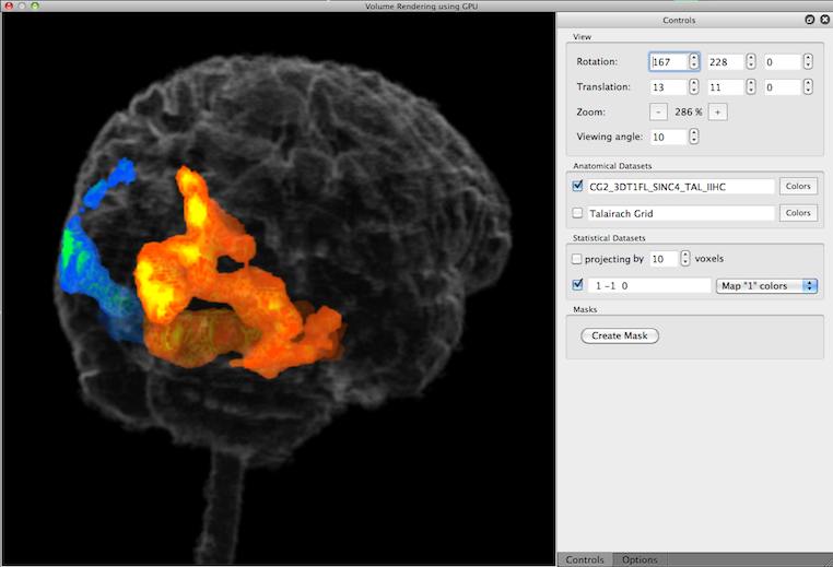
After re-launching the volume renderer with the modified VMR, the color dialog has been used to set the opacity component to a very low value (5%), i.e. the VMR has been made highly transparent. The rendered view now nicely shows how the functional activity is located within the brain; note that the map colors get shaded less vivid (more into black color) the further the activity is away from the boundary. A good impression of the true location of map data can be obtained when rotating the brain.
On the one hand such visualizations nicely extend the possibilities of the surface module that has other advantages including visualizations of morphed (inflated, flattened, spherical) cortex surfaces. If volume rendering is used without projection or transparancey, the resulting renderings look almost identical to the ones obtained with surface rendering.
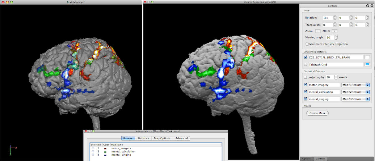
In the snapshot above, three maps were selected in the Volume Maps dialog prior to launching the volume renderer. The resulting rendering - without projection and transparency - looks very similar to a surface rendering shown on the left side using the same anatomical volume and volume maps.
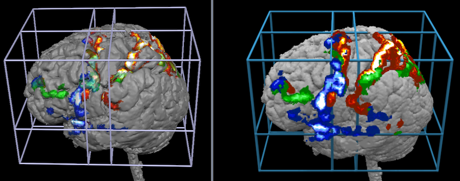
The snapshots above shows how volume rendering (right side) may add visualizations exploiting the projection option that was used here with a depth of 10 voxels. The snapshots below show how volume rendering may add visualizations when using transparency effects.
Additional rendering options including arbitrary cutting and shadow effects may be used to present anatomical and functional information with useful visualizations.
Copyright © 2014 Rainer Goebel. All rights reserved.