BrainVoyager QX v2.8
Group Analysis of Cortical Thickness Maps
Group-level analyses of cortical thickness measurements can be performed if the thickness surface maps of all included subjects have been computed for the cortically aligned cortex meshes. To calculate group average maps of cortical thickness or to compare the mapped thickness across groups, switch to the Group Maps tab of the Cortical Thickness Analysis dialog (see figure below). This tab contains a Groups field, which must be filled with a list of Thickness SMP files containing the individual thickness measurements. Depending on the created surface maps, you may run the group analyses twice, once for each hemisphere, or once for the whole cortex. Besides the thickness map entry, an SSM file must be provided for each subject describing the alignment of the individual cortex to the target (group) cortex. The SSM files are placed in the Cortex alignment SSM files column. The last column contains a Group identifier. Change the number to classify the subjects into different groups, for example, a healthy (1) and a patient group (2), by clicking an entry in the Group column. After editing the number, press the Return key to accept the new group identifier.
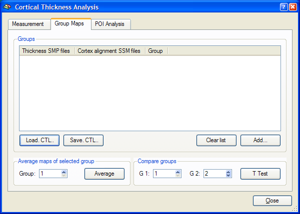
To add a subject to the list, click the Add button in the Groups field. The program will ask first for a thickness SMP file and then for the SSM file of the respective subject. If you made a mistake, you can delete individual entries by highlighting that entry and pressing the Delete key. If you want to remove all entries, click the Clear List button. You may also save an entered list to disk by clicking the Save .CTL button (CTL = cortical thickness group list). This is useful if you want to run the group analyses with a subset of subjects, which have been already scanned and prepared. When more subjects are available, you can click the Load .CTL button to load the previously saved list and then add new subjects using the Add button.
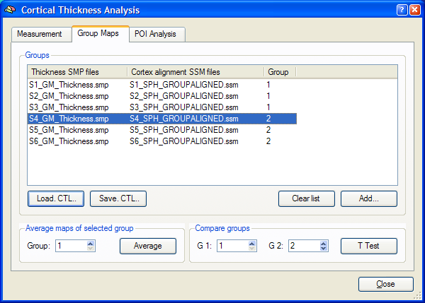
When you have added all subjects to the list, you can create an average map for a group of subjects as identified in the Group column. Use the Group spin box in the Average maps of selected group field to specify the group for averaging. If you want to create an average thickness map of all subjects of all groups, simply specify the same value (for example "1") for each subject in the Group column. To calculate the group average thickness map, click the Average button. The started calculation will average the thickness values from each subject at each vertex. Corresponding vertex indices are retrieved from the provided SSM files. It is recommended to overlay the resulting group thickness surface map on the target (group) cortex.
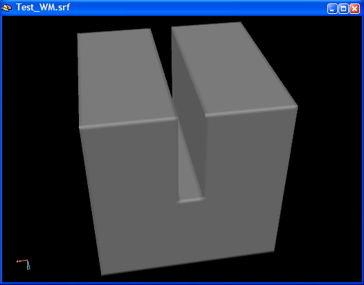
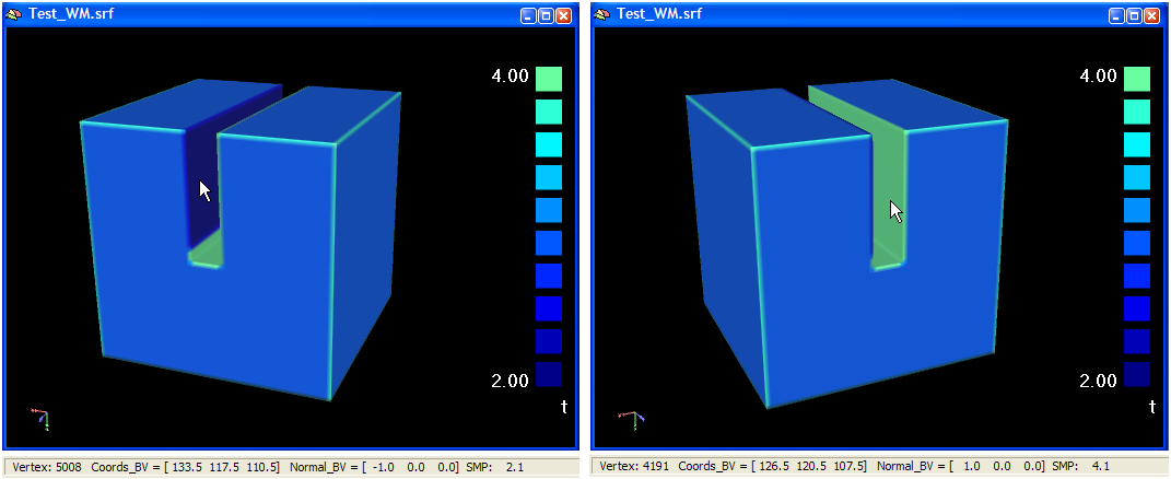
Note: The data used in this documentation section is from simulated data sets, which have been used to test the cortical thickness calculations. In the simulated data, a single sulcus has been modelled (see "white matter" surface in the figure above) with each bank of the sulcus with potentially different thickness values in the range of 2 to 5 mm. The figure below is the result of averaging the simulated data for group 2 (subjects S4 - S6). The thickness outside the sulcus is 3 mm (as simulated), but the average thickness of the two banks of the sulcus differs in group 2.
The figure below shows different colors for the two banks of the simulated sulcus indicating different thickness values. You can read the thickness value at any vertex precisely simply by Ctrl-clicking the mesh with the mouse pointer. This has been done at the two indicated positions in the figures below. The relevant information about the selected vertex is shown in the status bar, which has been copied below the snapshots in the figure below. Besides information about the coordinates of the vertex and its normal, the status bar shows values of the currently available surface maps. In our case, only one surface map is available, which is the averaged thickness map of group 2. Note that the selected vertex from the left bank of the sulcus (left part of the figure) shows a thickness value of 2.1 mm (SMP: 2.1), whereas the selected vertex from the right bank of the sulcus (right part of the figure) shows a thickness value of 4.1.
While the creation of average maps is important for visualization, it does not perform a statistical comparison between different groups. In order to map statistical differences in cortical thickness between groups, use the T Test button in the Compare groups field. The identifiers of the two groups to be compared can be specified with the G1 and G2 spin boxes. After clicking the T Test button, a group comparison is performed for each vertex separately calculating a standard t test:
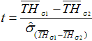
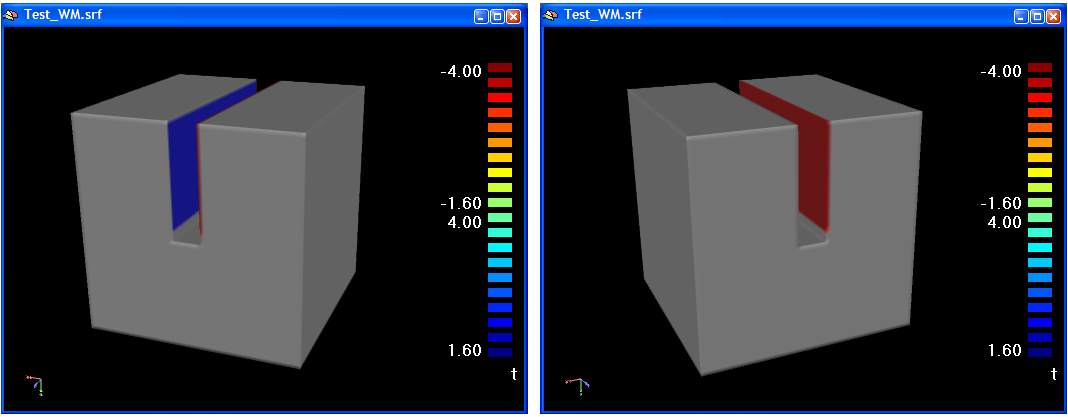
The symbol "TH" refers to a cortical thickness value. The numerator contains the difference of the mean cortical thickness of each of the two specified groups (at a vertex) and the denominator contains the standard error of this difference. Note that you need at least 2 subjects per group to run the calculation, but useful group comparisons will require at least 10 subjects per group (the more, the better). The computed t values, one for each vertex, are saved in the resulting t surface map, which is best visualized on the target (group) cortex. This group difference map will highlight those regions at which the two groups differ. You can increase / decrease as usual the critical map threshold to highlight regions with more or less significant differences. The t map showing the difference between the two groups for the simulated data is shown below. Since the thickness outside of the sulcus was the same for all subjects (3 mm), these regions are not color-coded. The thickness of the two banks, however, differ between the groups with group 1 having a thicker left bank and group 2 having a thicker right bank.
Copyright © 2014 Rainer Goebel. All rights reserved.