

Diffusion Tensor Imaging II
In the last part of this series, basic processing steps and calculations of useful DTI volume maps has been described. This part focuses on tensor visualization and fiber tracking as implemented in BrainVoyager QX 1.9. Tensor visualization and fiber tracking can be performed if a DDT file is available, which is itself derived from a corresponding VDW data set containing the original diffusion data in 3D space (original scanning space, AC-PC space or Talairach space). As described last time, the DDT file contains, for each voxel, the three estimated eigenvectors and associated eigenvalues describing the shape of a diffusion ellipsoid.
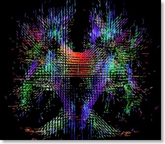
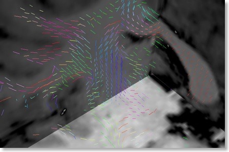
The orientation of the maximum eigenvector can be visualized as a line at the position of voxels in 3D space (see snapshot above) using the “Tensor Visualization” dialog, which can be called from the “DTI” menu. The dialog allows to change relevant display parameters, including a fractional anisotropy (FA) threshold value: The eigenvector is only shown if the FA value of the respective voxel surpasses the specified threshold. While providing important information, displaying orientation lines at all (supra-threshold) voxels may present a difficult to grasp visualizations, especially when low FA threshold values are used. To reduce this problem, the dialog contains an option allowing to restrict the display of eigenvectors to visualized slice planes (see snapshot below). When slowly slicing through the data, this approach provides direction data in combination with the underlying anatomy.
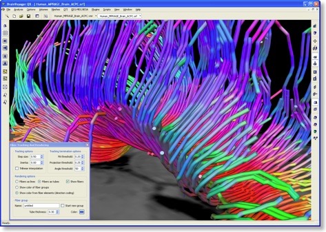
In order to explicitly visualize presumed fiber bundles, the eigenvector orientations in neighboring voxels have to be connected in a proper way. This connecting process (see snapshot below) is called “fiber tracking” and may lead to beautiful visualizations. Note that constructed fiber tracts may, however, not always properly reflect the true pathways of axonal fiber bundles because the diffusion data of each voxel constitutes a discrete, noisy sample of the average diffusion within a quite large region of space (e.g. a cube of 2 x 2 x 2 mm). The results of DTI fiber tracking, thus, requires careful interpretation.
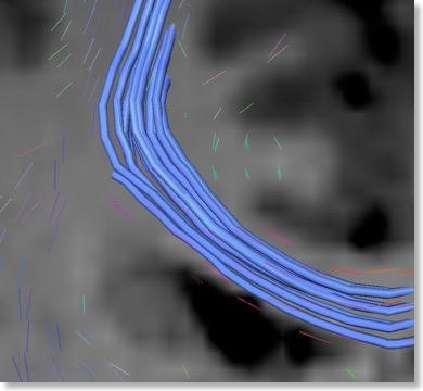
In BV QX 1.9, fibers can be tracked from anatomically or functionally defined volumes-of-interest (VOIs). The snapshot at the top of this blog was created using an anatomically defined VOI covering the corpus callosum on a mid-sagittal plane. For exploratory purposes, QX 1.9 supports real-time interactive fiber tracking. This requires only that one or more slice planes are turned on followed by a series of clicks on any desired region on one of the planes. Around the selected location, a set of sampled positions is used to define “seed points” for fiber tracking. Since the maximum eigenvector defines not a direction but specifies an orientation, tracking is performed in two opposing directions from each seed point. All fibers tracked from the seed points of a interactively selected position or a VOI are assembled within a fiber group. Each fiber group gets its own set of properties, including a color, a visibility flag (whether the fiber group should be shown or not) and a fiber thickness display parameter. The “Fiber Tracking and Rendering” dialog in combination with the “Fiber Table” dialog allow to select and change different display options. In order to allow real-time inspection (rotation, translation, zooming) of a large amount of fibers, one option allows to show fibers as lines. For more beautiful renderings, the “render as tubes” option can be selected. While rendering fiber groups in a specific color aids in keeping them apart, it is also possible to visualize small pieces of fibers in the color of the corresponding tensor orientation.
BrainVoyager QX 1.9 has now entered quality assurance testing and should be available in about 2-3 weeks from now.