

Diffusion Tensor Imaging I
The main new feature of BrainVoyager QX 1.9 is a comprehensive set of tools for the analysis of Diffusion Tensor Imaging (DTI) data. Since these tools are now nearly complete, I want to describe them in a short series of blog entries. First of all, I want to thank Alard Roebroeck for his excellent help. I used his software “TrackMark” as the model for my own development and decided early on to add an export function to save tensor calculations in TrackMark’s “TVL” file format. This allowed me to test my tools efficiently and it also makes sure that there will be an easy way to exchange data and tools between TrackMark and BrainVoyager QX in the future. I am also glad to let you know that we have a DTI specialist in our team at Brain Innovation, Pim Pullens. Pim will help me to further develop the DTI capabilities in BV QX and he will also be your prime contact person for questions concerning DTI analysis in BrainVoyager. At the moment, Pim is working on an advanced motion correction tool for diffusion weighted data.
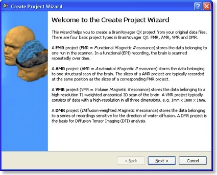
The DTI tools start with assembling raw diffusion data for all directions into a new project type, called DMR (“diffusion MR”). The raw data must contain at least one volume of non diffusion-weighted (b0) images and at least six volumes with diffusion measurements in six different directions. Recent DTI MR pulse sequences allow to scan many more diffusion directions (as well as several b0 volumes). A DMR project is created in BV QX 1.9 using the new “Create Project Wizard”. This new wizard is not limited to DMR projects, but can also be used to easily create FMR, VMR and AMR projects.
After the DMR has been created, the “DMR Properties” dialog pops up showing all essential information about the data, including number of volumes, number of slices and so on. Similarly as for FMR projects, the created DMR file does not contain the actual raw data, which is actually stored in a single “DWI” (diffusion weighted images) file. By pressing the “DWI Data” button, the “DWI Data” dialog (see below) is shown displaying the unique information of DMR projects.
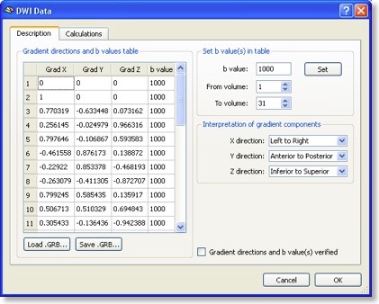
The most important information is the “Gradient directions and b values table” (see snapshot above) describing for each scanned volume the measured direction of diffusion as well as the used b value. In most DTI scans, the b value is the same for all directions. Each direction is specified by its associated x, y and z component. You may enter the values in the table or load a prepared text (“GRB”) file. You may also save the entered table, which is useful since the same direction table might be used for many scans. It is important that the diffusion direction table is interpreted in the right way, i.e. what direction is referred to by “x”, “y” and “z”. While the default assumptions made should be correct for most data sets, the interpretation can be adjusted in the “Interpretation of gradient components” field.
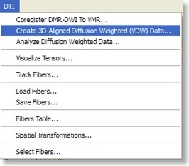
When the direction table has been defined, a diffusion tensor can be estimated at each voxel, which is the basis for calculation of useful maps as well as for fiber tracking. While estimation of tensors is possible already in the raw data space, it is recommended to transform the data in 3D space, e.g. AC-PC or Talairach space. The latter space is especially relevant for group comparisons of “FA” maps (see below), The steps to align the DWI data with a high-resolution 3D scan of the subject are identical to those used to align FMR and VMR data sets. The alignment routines are available in the new “DTI” menu (see snapshot above). When the “DMR” data has been aligned with a 3D data set, the actual “DWI” data is transformed into the new “VDW” (volumes of diffusion weighted data) format. A VDW file is similar to a VTC file except that it contains appropriate header information about the gradient table and a history of applied spatial transformations in order to allow correct interpretation of diffusion directions in any 3D space, including AC-PC and Talairach space.
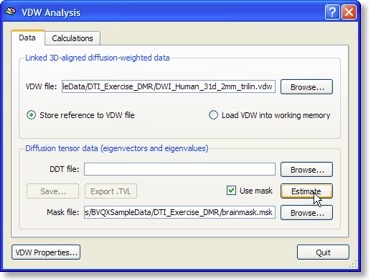
The “Analyze Diffusion Weighted Data” entry of the “DTI” menu calls the “VDW Analysis” dialog from which important calculations can be launched. As for the DMR-DWI data, the first essential calculation is the estimation of the diffusion tensors from the diffusion weighted (VDW) data (see snapshot above). For each voxel, the tensor estimation process results in three eigenvectors and associated eigenvalues. These quantities specify an ellipsoid characterizing the direction of diffusion and the amount of “anisotropy” (see below) in the respective voxel. The calculated tensor information is saved to disk as a “DDT” (diagonalized diffusion tensors) file for later reuse.
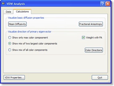
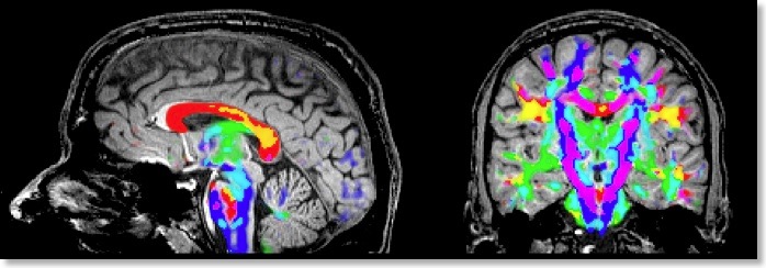
If all three eigenvectors of a voxel have an eigenvalue of similar magnitude, the diffusion is “isotropic” and the specified ellipsoid will be close to a sphere. If the eigenvalue of one eigenvector is large and the other two eigenvalues are small, diffusion is highly “anisotropic” and the ellipsoid will look like a cigar. The amount of anisotropy can thus be described by comparing the values of the three eigenvalues without using the eigenvectors (directions) themselves. The most common measure quantifying anisotropy is “Fractional Anisotropy” (FA) determining the fraction of the diffusion tensor, which can be ascribed to anisotropic diffusion. FA is calculated as a normalized variance of the three eigenvalues. The FA value varies between 0 (isotropic diffusion, looks like a sphere) and 1 (infinite anisotropy, looks like a line) The second row of the figure below shows a calculated FA map. The coronal slice nicely shows that anisotropy is high in white matter but low in grey matter. The three eigenvalues can also be used to calculate the overall amount of diffusion in a voxel. In a “mean diffusivity” (ADC) map, for example, all three eigenvalues are simply summed (or averaged). Row one of the figure above shows a mean diffusivity map clearly showing that diffusion is highest in cerebro-spinal fluid.
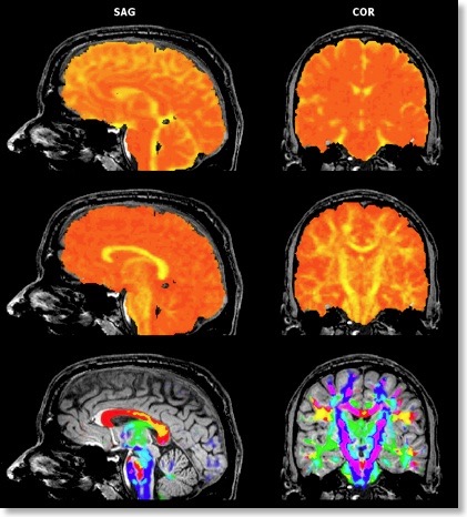
When using also the eigenvectors, color maps can be computed indicating the direction of diffusion. The most useful information is provided by the x, y and z components of the eigenvector with the largest eigenvalue. The color red, for example, can be used to indicate diffusion along the left/right axis (eigenvector [1, 0, 0] ), green for diffusion along the anterior/posterior axis (eigenvector [0, 1, 0] ) and blue for diffusion along the inferior/superior axis (eigenvector [0, 0, 1] ). Diffusion along intermediate directions can be visualized by appropriately mixing the three basic colors. Note that although an eigenvector points in a specific direction, the measured diffusion (of protons) occurs both along the direction of the eigenvector as well as in the opposing direction. An eigenvector thus must be interpreted as indicating an axis of diffusion.
The color direction map in the third row of the figure above only shows diffusion axes for voxels mainly confined to white matter. This is possible because BV QX allows to restrict calculations of the diffusion tensors to voxels specified in a mask (see snapshot of “VDW Analysis” dialog). As for masked statistical (GLM) analyses, a mask (.MSK) file can be created from a statistical map or from anatomical preprocessing steps, e.g. from the result of brain or white matter segmentation. Another option to restrict calculations to a useful subset of voxels is by enabling FA thresholding: Only voxels surpassing a given anisotropy threshold will be included in the color direction map. While the FA and mean diffusivity maps are stored as single maps, the color direction maps are stored as a set of three maps, each coding one component (x, y, z) of the maximum eigenvector. To optimize visualization, new options for mixing multiple maps have been introduced.